PyTorch Lightning


Lightning in 2 steps
In this guide we’ll show you how to organize your PyTorch code into Lightning in 2 steps.
Organizing your code with PyTorch Lightning makes your code:
Keep all the flexibility (this is all pure PyTorch), but removes a ton of boilerplate
More readable by decoupling the research code from the engineering
Easier to reproduce
Less error-prone by automating most of the training loop and tricky engineering
Scalable to any hardware without changing your model
Here’s a 3 minute conversion guide for PyTorch projects:
Step 0: Install PyTorch Lightning
You can install using pip
pip install pytorch-lightning
Or with conda (see how to install conda here):
conda install pytorch-lightning -c conda-forge
You could also use conda environments
conda activate my_env
pip install pytorch-lightning
Import the following:
import os
import torch
from torch import nn
import torch.nn.functional as F
from torchvision import transforms
from torchvision.datasets import MNIST
from torch.utils.data import DataLoader, random_split
import pytorch_lightning as pl
Step 1: Define LightningModule
class LitAutoEncoder(pl.LightningModule):
def __init__(self):
super().__init__()
self.encoder = nn.Sequential(nn.Linear(28 * 28, 64), nn.ReLU(), nn.Linear(64, 3))
self.decoder = nn.Sequential(nn.Linear(3, 64), nn.ReLU(), nn.Linear(64, 28 * 28))
def forward(self, x):
# in lightning, forward defines the prediction/inference actions
embedding = self.encoder(x)
return embedding
def training_step(self, batch, batch_idx):
# training_step defined the train loop.
# It is independent of forward
x, y = batch
x = x.view(x.size(0), -1)
z = self.encoder(x)
x_hat = self.decoder(z)
loss = F.mse_loss(x_hat, x)
# Logging to TensorBoard by default
self.log("train_loss", loss)
return loss
def configure_optimizers(self):
optimizer = torch.optim.Adam(self.parameters(), lr=1e-3)
return optimizer
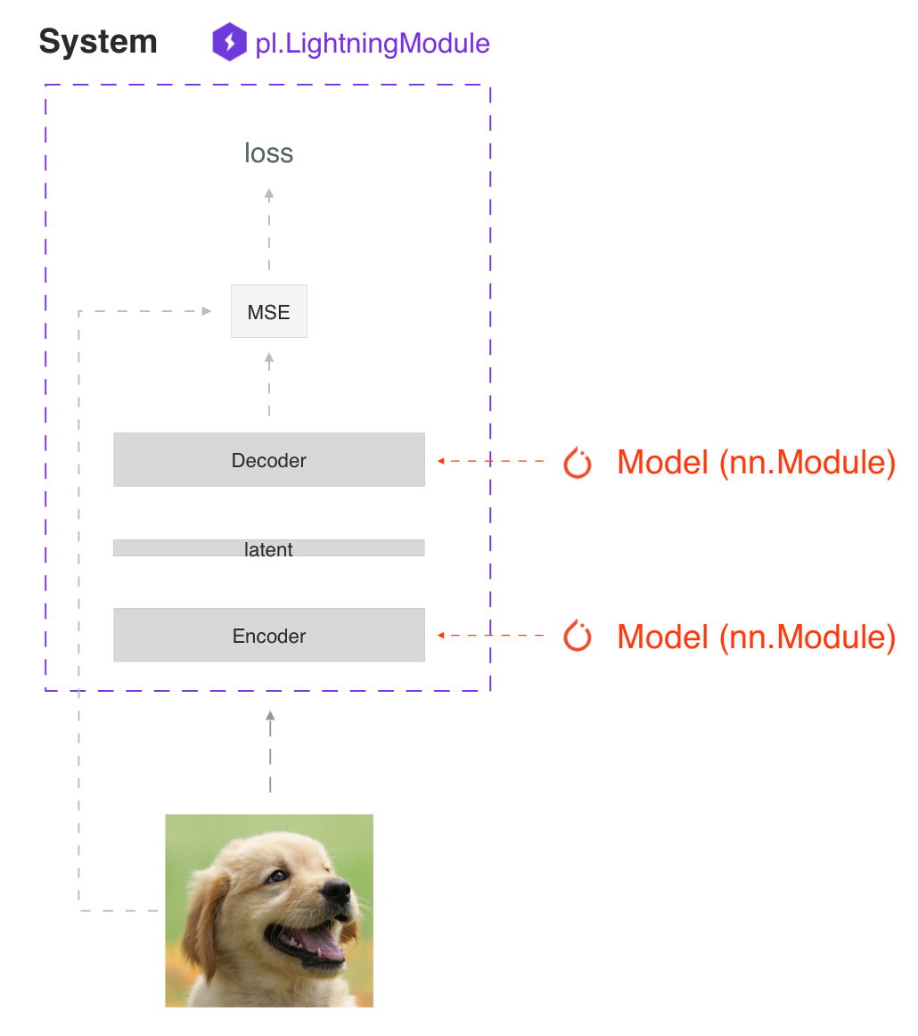
SYSTEM VS MODEL
A lightning module defines a system not a model.
Examples of systems are:
Seq2seq
Under the hood a LightningModule is still just a torch.nn.Module that groups all research code into a single file to make it self-contained:
The Train loop
The Validation loop
The Test loop
The Prediction loop
The Model or system of Models
The Optimizer
You can customize any part of training (such as the backward pass) by overriding any of the 20+ hooks found in Available Callback hooks
class LitAutoEncoder(LightningModule):
def backward(self, loss, optimizer, optimizer_idx):
loss.backward()
FORWARD vs TRAINING_STEP
In Lightning we separate training from inference. The training_step defines the full training loop. We encourage users to use the forward to define inference actions.
For example, in this case we could define the autoencoder to act as an embedding extractor:
def forward(self, x):
embeddings = self.encoder(x)
return embeddings
Of course, nothing is stopping you from using forward from within the training_step.
def training_step(self, batch, batch_idx):
...
z = self(x)
It really comes down to your application. We do, however, recommend that you keep both intents separate.
Use forward for inference (predicting).
Use training_step for training.
More details in lightning module docs.
Step 2: Fit with Lightning Trainer
First, define the data however you want. Lightning just needs a DataLoader for the train/val/test/predict splits.
dataset = MNIST(os.getcwd(), download=True, transform=transforms.ToTensor())
train_loader = DataLoader(dataset)
Next, init the lightning module and the PyTorch Lightning Trainer,
then call fit with both the data and model.
# init model
autoencoder = LitAutoEncoder()
# most basic trainer, uses good defaults (auto-tensorboard, checkpoints, logs, and more)
# trainer = pl.Trainer(gpus=8) (if you have GPUs)
trainer = pl.Trainer()
trainer.fit(autoencoder, train_loader)
The Trainer automates:
Epoch and batch iteration
Calling of optimizer.step(), backward, zero_grad()
Calling of .eval(), enabling/disabling grads
Tensorboard (see loggers options)
Multi-GPU support
16-bit precision AMP support
Tip
If you prefer to manually manage optimizers you can use the Manual optimization mode (ie: RL, GANs, etc…).
That’s it!
These are the main 2 concepts you need to know in Lightning. All the other features of lightning are either features of the Trainer or LightningModule.
Basic features
Manual vs automatic optimization
Automatic optimization
With Lightning, you don’t need to worry about when to enable/disable grads, do a backward pass, or update optimizers as long as you return a loss with an attached graph from the training_step, Lightning will automate the optimization.
def training_step(self, batch, batch_idx):
loss = self.encoder(batch)
return loss
Manual optimization
However, for certain research like GANs, reinforcement learning, or something with multiple optimizers or an inner loop, you can turn off automatic optimization and fully control the training loop yourself.
Turn off automatic optimization and you control the train loop!
def __init__(self):
self.automatic_optimization = False
def training_step(self, batch, batch_idx):
# access your optimizers with use_pl_optimizer=False. Default is True,
# setting use_pl_optimizer=True will maintain plugin/precision support
opt_a, opt_b = self.optimizers(use_pl_optimizer=True)
loss_a = self.generator(batch)
opt_a.zero_grad()
# use `manual_backward()` instead of `loss.backward` to automate half precision, etc...
self.manual_backward(loss_a)
opt_a.step()
loss_b = self.discriminator(batch)
opt_b.zero_grad()
self.manual_backward(loss_b)
opt_b.step()
Loop customization
If you need even more flexibility, you can fully customize the training loop to its core. Learn more about loops here.
Predict or Deploy
When you’re done training, you have 3 options to use your LightningModule for predictions.
Option 1: Sub-models
Pull out any model inside your system for predictions.
# ----------------------------------
# to use as embedding extractor
# ----------------------------------
autoencoder = LitAutoEncoder.load_from_checkpoint("path/to/checkpoint_file.ckpt")
encoder_model = autoencoder.encoder
encoder_model.eval()
# ----------------------------------
# to use as image generator
# ----------------------------------
decoder_model = autoencoder.decoder
decoder_model.eval()
Option 2: Forward
You can also add a forward method to do predictions however you want.
# ----------------------------------
# using the AE to extract embeddings
# ----------------------------------
class LitAutoEncoder(LightningModule):
def __init__(self):
super().__init__()
self.encoder = nn.Sequential()
def forward(self, x):
embedding = self.encoder(x)
return embedding
autoencoder = LitAutoEncoder()
embedding = autoencoder(torch.rand(1, 28 * 28))
# ----------------------------------
# or using the AE to generate images
# ----------------------------------
class LitAutoEncoder(LightningModule):
def __init__(self):
super().__init__()
self.decoder = nn.Sequential()
def forward(self):
z = torch.rand(1, 3)
image = self.decoder(z)
image = image.view(1, 1, 28, 28)
return image
autoencoder = LitAutoEncoder()
image_sample = autoencoder()
Option 3: Production
For production systems, onnx or torchscript are much faster. Make sure you have added a forward method or trace only the sub-models you need.
# ----------------------------------
# torchscript
# ----------------------------------
autoencoder = LitAutoEncoder()
torch.jit.save(autoencoder.to_torchscript(), "model.pt")
os.path.isfile("model.pt")
# ----------------------------------
# onnx
# ----------------------------------
with tempfile.NamedTemporaryFile(suffix=".onnx", delete=False) as tmpfile:
autoencoder = LitAutoEncoder()
input_sample = torch.randn((1, 28 * 28))
autoencoder.to_onnx(tmpfile.name, input_sample, export_params=True)
os.path.isfile(tmpfile.name)
Using CPUs/GPUs/TPUs/IPUs
It’s trivial to use CPUs, GPUs, TPUs or IPUs in Lightning. There’s NO NEED to change your code, simply change the Trainer options.
# train on CPU
trainer = Trainer()
# train on 8 CPUs
trainer = Trainer(num_processes=8)
# train on 1024 CPUs across 128 machines
trainer = pl.Trainer(num_processes=8, num_nodes=128)
# train on 1 GPU
trainer = pl.Trainer(gpus=1)
# train on multiple GPUs across nodes (32 gpus here)
trainer = pl.Trainer(gpus=4, num_nodes=8)
# train on gpu 1, 3, 5 (3 gpus total)
trainer = pl.Trainer(gpus=[1, 3, 5])
# Multi GPU with mixed precision
trainer = pl.Trainer(gpus=2, precision=16)
# Train on TPUs
trainer = pl.Trainer(tpu_cores=8)
Without changing a SINGLE line of your code, you can now do the following with the above code:
# train on TPUs using 16 bit precision
# using only half the training data and checking validation every quarter of a training epoch
trainer = pl.Trainer(tpu_cores=8, precision=16, limit_train_batches=0.5, val_check_interval=0.25)
# Train on IPUs
trainer = pl.Trainer(ipus=8)
Checkpoints
Lightning automatically saves your model. Once you’ve trained, you can load the checkpoints as follows:
model = LitModel.load_from_checkpoint(path)
The above checkpoint contains all the arguments needed to init the model and set the state dict. If you prefer to do it manually, here’s the equivalent
# load the ckpt
ckpt = torch.load("path/to/checkpoint.ckpt")
# equivalent to the above
model = LitModel()
model.load_state_dict(ckpt["state_dict"])
Data flow
Each loop (training, validation, test, predict) has three hooks you can implement:
x_step
x_step_end
x_epoch_end
To illustrate how data flows, we’ll use the training loop (ie: x=training)
outs = []
for batch in data:
out = training_step(batch)
outs.append(out)
training_epoch_end(outs)
The equivalent in Lightning is:
def training_step(self, batch, batch_idx):
prediction = ...
return prediction
def training_epoch_end(self, outs):
for out in outs:
...
In the event that you use DP or DDP2 distributed modes (ie: split a batch across GPUs), use the x_step_end to manually aggregate (or don’t implement it to let lightning auto-aggregate for you).
for batch in data:
model_copies = copy_model_per_gpu(model, num_gpus)
batch_split = split_batch_per_gpu(batch, num_gpus)
gpu_outs = []
for model, batch_part in zip(model_copies, batch_split):
# LightningModule hook
gpu_out = model.training_step(batch_part)
gpu_outs.append(gpu_out)
# LightningModule hook
out = training_step_end(gpu_outs)
The lightning equivalent is:
def training_step(self, batch, batch_idx):
loss = ...
return loss
def training_step_end(self, losses):
gpu_0_loss = losses[0]
gpu_1_loss = losses[1]
return (gpu_0_loss + gpu_1_loss) / 2
Tip
The validation, test and prediction loops have the same structure.
Logging
To log to Tensorboard, your favorite logger, and/or the progress bar, use the
log() method which can be called from
any method in the LightningModule.
def training_step(self, batch, batch_idx):
self.log("my_metric", x)
The log() method has a few options:
on_step (logs the metric at that step in training)
on_epoch (automatically accumulates and logs at the end of the epoch)
prog_bar (logs to the progress bar)
logger (logs to the logger like Tensorboard)
Depending on where the log is called from, Lightning auto-determines the correct mode for you. But of course you can override the default behavior by manually setting the flags
Note
Setting on_epoch=True will accumulate your logged values over the full training epoch.
def training_step(self, batch, batch_idx):
self.log("my_loss", loss, on_step=True, on_epoch=True, prog_bar=True, logger=True)
Note
The loss value shown in the progress bar is smoothed (averaged) over the last values, so it differs from the actual loss returned in the train/validation step.
You can also use any method of your logger directly:
def training_step(self, batch, batch_idx):
tensorboard = self.logger.experiment
tensorboard.any_summary_writer_method_you_want()
Once your training starts, you can view the logs by using your favorite logger or booting up the Tensorboard logs:
tensorboard --logdir ./lightning_logs
Note
Lightning automatically shows the loss value returned from training_step in the progress bar.
So, no need to explicitly log like this self.log('loss', loss, prog_bar=True).
Read more about loggers.
Optional extensions
Callbacks
A callback is an arbitrary self-contained program that can be executed at arbitrary parts of the training loop.
Here’s an example adding a not-so-fancy learning rate decay rule:
from pytorch_lightning.callbacks import Callback
class DecayLearningRate(Callback):
def __init__(self):
self.old_lrs = []
def on_train_start(self, trainer, pl_module):
# track the initial learning rates
for opt_idx, optimizer in enumerate(trainer.optimizers):
group = [param_group["lr"] for param_group in optimizer.param_groups]
self.old_lrs.append(group)
def on_train_epoch_end(self, trainer, pl_module):
for opt_idx, optimizer in enumerate(trainer.optimizers):
old_lr_group = self.old_lrs[opt_idx]
new_lr_group = []
for p_idx, param_group in enumerate(optimizer.param_groups):
old_lr = old_lr_group[p_idx]
new_lr = old_lr * 0.98
new_lr_group.append(new_lr)
param_group["lr"] = new_lr
self.old_lrs[opt_idx] = new_lr_group
# And pass the callback to the Trainer
decay_callback = DecayLearningRate()
trainer = Trainer(callbacks=[decay_callback])
Things you can do with a callback:
Send emails at some point in training
Grow the model
Update learning rates
Visualize gradients
…
You are only limited by your imagination
LightningDataModules
DataLoaders and data processing code tends to end up scattered around.
Make your data code reusable by organizing it into a LightningDataModule.
class MNISTDataModule(LightningDataModule):
def __init__(self, batch_size=32):
super().__init__()
self.batch_size = batch_size
# When doing distributed training, Datamodules have two optional arguments for
# granular control over download/prepare/splitting data:
# OPTIONAL, called only on 1 GPU/machine
def prepare_data(self):
MNIST(os.getcwd(), train=True, download=True)
MNIST(os.getcwd(), train=False, download=True)
# OPTIONAL, called for every GPU/machine (assigning state is OK)
def setup(self, stage: Optional[str] = None):
# transforms
transform = transforms.Compose([transforms.ToTensor(), transforms.Normalize((0.1307,), (0.3081,))])
# split dataset
if stage in (None, "fit"):
mnist_train = MNIST(os.getcwd(), train=True, transform=transform)
self.mnist_train, self.mnist_val = random_split(mnist_train, [55000, 5000])
if stage == "test":
self.mnist_test = MNIST(os.getcwd(), train=False, transform=transform)
if stage == "predict":
self.mnist_predict = MNIST(os.getcwd(), train=False, transform=transform)
# return the dataloader for each split
def train_dataloader(self):
mnist_train = DataLoader(self.mnist_train, batch_size=self.batch_size)
return mnist_train
def val_dataloader(self):
mnist_val = DataLoader(self.mnist_val, batch_size=self.batch_size)
return mnist_val
def test_dataloader(self):
mnist_test = DataLoader(self.mnist_test, batch_size=self.batch_size)
return mnist_test
def predict_dataloader(self):
mnist_predict = DataLoader(self.mnist_predict, batch_size=self.batch_size)
return mnist_predict
LightningDataModule is designed to enable sharing and reusing data splits
and transforms across different projects. It encapsulates all the steps needed to process data: downloading,
tokenizing, processing etc.
Now you can simply pass your LightningDataModule to
the Trainer:
# init model
model = LitModel()
# init data
dm = MNISTDataModule()
# train
trainer = pl.Trainer()
trainer.fit(model, datamodule=dm)
# validate
trainer.validate(datamodule=dm)
# test
trainer.test(datamodule=dm)
# predict
predictions = trainer.predict(datamodule=dm)
DataModules are specifically useful for building models based on data. Read more on datamodules.
Debugging
Lightning has many tools for debugging. Here is an example of just a few of them:
# use only 10 train batches and 3 val batches
trainer = Trainer(limit_train_batches=10, limit_val_batches=3)
# Automatically overfit the same batch of your model for a sanity test
trainer = Trainer(overfit_batches=1)
# unit test all the code - hits every line of your code once to see if you have bugs,
# instead of waiting hours to crash on validation
trainer = Trainer(fast_dev_run=True)
# unit test all the code - hits every line of your code with 4 batches
trainer = Trainer(fast_dev_run=4)
# train only 20% of an epoch
trainer = Trainer(limit_train_batches=0.2)
# run validation every 25% of a training epoch
trainer = Trainer(val_check_interval=0.25)
# Profile your code to find speed/memory bottlenecks
Trainer(profiler="simple")
Other cool features
Once you define and train your first Lightning model, you might want to try other cool features like
Or read our Guide to learn more!
Grid AI
Grid AI is our native solution for large scale training and tuning on the cloud.
Get started for free with your GitHub or Google Account here.
Community
Our community of core maintainers and thousands of expert researchers is active on our Slack and GitHub Discussions. Drop by to hang out, ask Lightning questions or even discuss research!
Masterclass
We also offer a Masterclass to teach you the advanced uses of Lightning.

How to organize PyTorch into Lightning
To enable your code to work with Lightning, here’s how to organize PyTorch into Lightning
1. Move your computational code
Move the model architecture and forward pass to your lightning module.
class LitModel(LightningModule):
def __init__(self):
super().__init__()
self.layer_1 = nn.Linear(28 * 28, 128)
self.layer_2 = nn.Linear(128, 10)
def forward(self, x):
x = x.view(x.size(0), -1)
x = self.layer_1(x)
x = F.relu(x)
x = self.layer_2(x)
return x
2. Move the optimizer(s) and schedulers
Move your optimizers to the configure_optimizers() hook.
class LitModel(LightningModule):
def configure_optimizers(self):
optimizer = torch.optim.Adam(self.parameters(), lr=1e-3)
return optimizer
3. Find the train loop “meat”
Lightning automates most of the training for you, the epoch and batch iterations, all you need to keep is the training step logic.
This should go into the training_step() hook (make sure to use the hook parameters, batch and batch_idx in this case):
class LitModel(LightningModule):
def training_step(self, batch, batch_idx):
x, y = batch
y_hat = self(x)
loss = F.cross_entropy(y_hat, y)
return loss
4. Find the val loop “meat”
To add an (optional) validation loop add logic to the
validation_step() hook (make sure to use the hook parameters, batch and batch_idx in this case).
class LitModel(LightningModule):
def validation_step(self, batch, batch_idx):
x, y = batch
y_hat = self(x)
val_loss = F.cross_entropy(y_hat, y)
return val_loss
Note
model.eval() and torch.no_grad() are called automatically for validation
5. Find the test loop “meat”
To add an (optional) test loop add logic to the
test_step() hook (make sure to use the hook parameters, batch and batch_idx in this case).
class LitModel(LightningModule):
def test_step(self, batch, batch_idx):
x, y = batch
y_hat = self(x)
loss = F.cross_entropy(y_hat, y)
return loss
Note
model.eval() and torch.no_grad() are called automatically for testing.
The test loop will not be used until you call.
trainer.test()
Tip
.test() loads the best checkpoint automatically
6. Remove any .cuda() or to.device() calls
Your lightning module can automatically run on any hardware!
Rapid prototyping templates
Use these templates for rapid prototyping
General Use
Use case |
Description |
link |
|---|---|---|
Scratch model |
To prototype quickly / debug with random data |
|
Scratch model with manual optimization |
To prototype quickly / debug with random data |
LightningLite - Stepping Stone to Lightning
LightningLite enables pure PyTorch users to scale their existing code
on any kind of device while retaining full control over their own loops and optimization logic.

LightningLite is the right tool for you if you match one of the two following descriptions:
I want to quickly scale my existing code to multiple devices with minimal code changes.
I would like to convert my existing code to the Lightning API, but a full path to Lightning transition might be too complex. I am looking for a stepping stone to ensure reproducibility during the transition.
Warning
LightningLite is currently a beta feature. Its API is subject to change based on your feedbacks.
Learn by example
My existing PyTorch code
The run function contains custom training loop used to train MyModel on MyDataset for num_epochs epochs.
import torch
from torch import nn
from torch.utils.data import DataLoader, Dataset
class MyModel(nn.Module):
...
class MyDataset(Dataset):
...
def run(args):
device = "cuda" if torch.cuda.is_available() else "cpu"
model = MyModel(...).to(device)
optimizer = torch.optim.SGD(model.parameters(), ...)
dataloader = DataLoader(MyDataset(...), ...)
model.train()
for epoch in range(args.num_epochs):
for batch in dataloader:
batch = batch.to(device)
optimizer.zero_grad()
loss = model(batch)
loss.backward()
optimizer.step()
run(args)
Convert to LightningLite
Here are 5 required steps to convert to LightningLite.
Subclass
LightningLiteand override itsrun()method.Move the body of your existing
runfunction intoLightningLiterunmethod.Remove all
.to,.cudaetc calls sinceLightningLitewill take care of it.Apply
setup()over each model and optimizers pair andsetup_dataloaders()on all your dataloaders and replaceloss.backward()byself.backward(loss).Instantiate your
LightningLiteand call itsrun()method.
import torch
from torch import nn
from torch.utils.data import DataLoader, Dataset
from pytorch_lightning.lite import LightningLite
class MyModel(nn.Module):
...
class MyDataset(Dataset):
...
class Lite(LightningLite):
def run(self, args):
model = MyModel(...)
optimizer = torch.optim.SGD(model.parameters(), ...)
model, optimizer = self.setup(model, optimizer) # Scale your model / optimizers
dataloader = DataLoader(MyDataset(...), ...)
dataloader = self.setup_dataloaders(dataloader) # Scale your dataloaders
model.train()
for epoch in range(args.num_epochs):
for batch in dataloader:
optimizer.zero_grad()
loss = model(batch)
self.backward(loss) # instead of loss.backward()
optimizer.step()
Lite(...).run(args)
That’s all. You can now train on any kind of device and scale your training.
The LightningLite takes care of device management, so you don’t have to.
You should remove any device specific logic within your code.
Here is how to train on 8 GPUs with torch.bfloat16 precision:
Lite(strategy="ddp", devices=8, accelerator="gpu", precision="bf16").run(10)
Here is how to use DeepSpeed Zero3 with 8 GPUs and precision 16:
Lite(strategy="deepspeed", devices=8, accelerator="gpu", precision=16).run(10)
LightningLite can also figure it out automatically for you!
Lite(devices="auto", accelerator="auto", precision=16).run(10)
You can also easily use distributed collectives if required. Here is an example while running on 256 GPUs.
class Lite(LightningLite):
def run(self):
# Transfer and concatenate tensors across processes
self.all_gather(...)
# Transfer an object from one process to all the others
self.broadcast(..., src=...)
# The total number of processes running across all devices and nodes.
self.world_size
# The global index of the current process across all devices and nodes.
self.global_rank
# The index of the current process among the processes running on the local node.
self.local_rank
# The index of the current node.
self.node_rank
# Wether this global rank is rank zero.
if self.is_global_zero:
# do something on rank 0
...
# Wait for all processes to enter this call.
self.barrier()
Lite(strategy="ddp", gpus=8, num_nodes=32, accelerator="gpu").run()
If you require custom data or model device placement, you can deactivate
LightningLite automatic placement by doing
self.setup_dataloaders(..., move_to_device=False) for the data and
self.setup(..., move_to_device=False) for the model.
Futhermore, you can access the current device from self.device or
rely on to_device()
utility to move an object to the current device.
Note
We recommend instantiating the models within the run() method as large models would cause an out-of-memory error otherwise.
Note
If you have hundreds or thousands of line within your run() function
and you are feeling weird about it then this is right feeling.
Back in 2019, our LightningModule was getting larger
and we got the same feeling. So we started to organize our code for simplicity, interoperability and standardization.
This is definitely a good sign that you should consider refactoring your code and / or switch to
LightningModule ultimately.
Distributed Training Pitfalls
The LightningLite provides you only with the tool to scale your training,
but there are several major challenges ahead of you now:
Processes divergence |
This happens when processes execute a different section of the code due to different if/else conditions, race condition on existing files, etc., resulting in hanging. |
Cross processes reduction |
Wrongly reported metrics or gradients due to mis-reduction. |
Large sharded models |
Instantiation, materialization and state management of large models. |
Rank 0 only actions |
Logging, profiling, etc. |
Checkpointing / Early stopping / Callbacks / Logging |
Ability to easily customize your training behaviour and make it stateful. |
Batch-level fault tolerance training |
Ability to resume from a failure as if it never happened. |
If you are facing one of those challenges then you are already meeting the limit of LightningLite.
We recommend you to convert to Lightning, so you never have to worry about those.
Convert to Lightning
The LightningLite is a stepping stone to transition fully to the Lightning API and benefits
from its hundreds of features.
You can see our LightningLite as a
future LightningModule and slowly refactor your code into its API.
Below, the training_step(), forward(),
configure_optimizers(), train_dataloader()
are being implemented.
class Lite(LightningLite):
# 1. This would becomes the LightningModule `__init__` function.
def run(self, args):
self.args = args
self.model = MyModel(...)
self.fit() # This would be automated by Lightning Trainer.
# 2. This can be fully removed as Lightning handles the FitLoop
# and setting up the model, optimizer, dataloader and many more.
def fit(self):
# setting everything
optimizer = self.configure_optimizers()
self.model, optimizer = self.setup(self.model, optimizer)
dataloader = self.setup_dataloaders(self.train_dataloader())
# start fitting
self.model.train()
for epoch in range(num_epochs):
for batch in enumerate(dataloader):
optimizer.zero_grad()
loss = self.training_step(batch, batch_idx)
self.backward(loss)
optimizer.step()
# 3. This stays here as it belongs to the LightningModule.
def forward(self, x):
return self.model(x)
def training_step(self, batch, batch_idx):
return self.forward(batch)
def configure_optimizers(self):
return torch.optim.SGD(self.model.parameters(), ...)
# 4. [Optionally] This can stay here or be extracted within a LightningDataModule to enable higher composability.
def train_dataloader(self):
return DataLoader(MyDataset(...), ...)
Lite(...).run(args)
Finally, change the run() into a
__init__() and drop the fit method.
from pytorch_lightning import LightningDataModule, LightningModule, Trainer
class LightningModel(LightningModule):
def __init__(self, args):
super().__init__()
self.model = MyModel(...)
def forward(self, x):
return self.model(x)
def training_step(self, batch, batch_idx):
loss = self(batch)
self.log("train_loss", loss)
return loss
def configure_optimizers(self):
return torch.optim.SGD(self.model.parameters(), lr=0.001)
class BoringDataModule(LightningDataModule):
def train_dataloader(self):
return DataLoader(MyDataset(...), ...)
trainer = Trainer(max_epochs=10)
trainer.fit(LightningModel(), datamodule=BoringDataModule())
You have successfully converted to PyTorch Lightning and can now benefit from its hundred of features !
Lightning Lite Flags
Lite is a specialist for accelerated distributed training and inference. It offers you convenient ways to configure your device and communication strategy and to seamlessly switch from one to the other. The terminology and usage is identical to Lightning, which means minimum effort for you to convert when you decide to do so.
accelerator
Choose one of "cpu", "gpu", "tpu", "auto" (IPU support is coming soon).
# CPU accelerator
lite = Lite(accelerator="cpu")
# Running with GPU Accelerator using 2 GPUs
lite = Lite(devices=2, accelerator="gpu")
# Running with TPU Accelerator using 8 tpu cores
lite = Lite(devices=8, accelerator="tpu")
# Running with GPU Accelerator using the DistributedDataParallel strategy
lite = Lite(devices=4, accelerator="gpu", strategy="ddp")
The "auto" option recognizes the machine you are on, and selects the available accelerator.
# If your machine has GPUs, it will use the GPU Accelerator
lite = Lite(devices=2, accelerator="auto")
strategy
Choose a training strategy: "dp", "ddp", "ddp_spawn", "tpu_spawn", "deepspeed", "ddp_sharded", or "ddp_sharded_spawn".
# Running with the DistributedDataParallel strategy on 4 GPUs
lite = Lite(strategy="ddp", accelerator="gpu", devices=4)
# Running with the DDP Spawn strategy using 4 cpu processes
lite = Lite(strategy="ddp_spawn", accelerator="cpu", devices=4)
Additionally, you can pass in your custom training type strategy by configuring additional parameters.
from pytorch_lightning.plugins import DeepSpeedPlugin
lite = Lite(strategy=DeepSpeedPlugin(stage=2), accelerator="gpu", devices=2)
Support for Horovod and Fully Sharded training strategies are coming soon.
devices
Configure the devices to run on. Can be of type:
int: the number of devices (e.g., GPUs) to train on
list of int: which device index (e.g., GPU ID) to train on (0-indexed)
str: a string representation of one of the above
# default used by Lite, i.e., use the CPU
lite = Lite(devices=None)
# equivalent
lite = Lite(devices=0)
# int: run on 2 GPUs
lite = Lite(devices=2, accelerator="gpu")
# list: run on GPUs 1, 4 (by bus ordering)
lite = Lite(devices=[1, 4], accelerator="gpu")
lite = Lite(devices="1, 4", accelerator="gpu") # equivalent
# -1: run on all GPUs
lite = Lite(devices=-1, accelerator="gpu")
lite = Lite(devices="-1", accelerator="gpu") # equivalent
gpus
Shorthand for setting devices=X and accelerator="gpu".
# Run on 2 GPUs
lite = Lite(gpus=2)
# Equivalent
lite = Lite(devices=2, accelerator="gpu")
tpu_cores
Shorthand for devices=X and accelerator="tpu".
# Run on 8 TPUs
lite = Lite(tpu_cores=8)
# Equivalent
lite = Lite(devices=8, accelerator="tpu")
num_nodes
Number of cluster nodes for distributed operation.
# Default used by Lite
lite = Lite(num_nodes=1)
# Run on 8 nodes
lite = Lite(num_nodes=8)
Learn more about distributed multi-node training on clusters here.
precision
Lightning Lite supports double precision (64), full precision (32), or half precision (16) operation (including bfloat16). Half precision, or mixed precision, is the combined use of 32 and 16 bit floating points to reduce the memory footprint during model training. This can result in improved performance, achieving significant speedups on modern GPUs.
# Default used by the Lite
lite = Lite(precision=32, devices=1)
# 16-bit (mixed) precision
lite = Lite(precision=16, devices=1)
# 16-bit bfloat precision
lite = Lite(precision="bf16", devices=1)
# 64-bit (double) precision
lite = Lite(precision=64, devices=1)
plugins
Plugins allow you to connect arbitrary backends, precision libraries, clusters etc. For example:
To define your own behavior, subclass the relevant class and pass it in. Here’s an example linking up your own
ClusterEnvironment.
from pytorch_lightning.plugins.environments import ClusterEnvironment
class MyCluster(ClusterEnvironment):
@property
def main_address(self):
return your_main_address
@property
def main_port(self):
return your_main_port
def world_size(self):
return the_world_size
lite = Lite(plugins=[MyCluster()], ...)
Lightning Lite Methods
run
The run method servers two purposes:
Override this method from the
LightningLiteclass and put your training (or inference) code inside.Launch the training by calling the run method. Lite will take care of setting up the distributed backend.
You can optionally pass arguments to the run method. For example, the hyperparameters or a backbone for the model.
from pytorch_lightning.lite import LightningLite
class Lite(LightningLite):
# Input arguments are optional, put whatever you need
def run(self, learning_rate, num_layers):
"""Here goes your training loop"""
lite = Lite(accelerator="gpu", devices=2)
lite.run(learning_rate=0.01, num_layers=12)
setup
Setup a model and corresponding optimizer(s). If you need to setup multiple models, call setup() on each of them.
Moves the model and optimizer to the correct device automatically.
model = nn.Linear(32, 64)
optimizer = torch.optim.SGD(model.parameters(), lr=0.001)
# Setup model and optimizer for accelerated training
model, optimizer = self.setup(model, optimizer)
# If you don't want Lite to set the device
model, optimizer = self.setup(model, optimizer, move_to_device=False)
The setup method also prepares the model for the selected precision choice so that operations during forward() get
cast automatically.
setup_dataloaders
Setup one or multiple dataloaders for accelerated operation. If you are running a distributed strategy (e.g., DDP), Lite will replace the sampler automatically for you. In addition, the dataloader will be configured to move the returned data tensors to the correct device automatically.
train_data = torch.utils.DataLoader(train_dataset, ...)
test_data = torch.utils.DataLoader(test_dataset, ...)
train_data, test_data = self.setup_dataloaders(train_data, test_data)
# If you don't want Lite to move the data to the device
train_data, test_data = self.setup_dataloaders(train_data, test_data, move_to_device=False)
# If you don't want Lite to replace the sampler in the context of distributed training
train_data, test_data = self.setup_dataloaders(train_data, test_data, replace_sampler=False)
backward
This replaces any occurences of loss.backward() and will make your code accelerator and precision agnostic.
output = model(input)
loss = loss_fn(output, target)
# loss.backward()
self.backward(loss)
to_device
Use to_device() to move models, tensors or collections of tensors to
the current device. By default setup() and
setup_dataloaders() already move the model and data to the correct
device, so calling this method is only necessary for manual operation when needed.
data = torch.load("dataset.pt")
data = self.to_device(data)
seed_everything
Make your code reproducible by calling this method at the beginning of your run.
# Instead of `torch.manual_seed(...)`, call:
self.seed_everything(1234)
This covers PyTorch, NumPy and Python random number generators. In addition, Lite takes care of properly initializing
the seed of dataloader worker processes (can be turned off by passing workers=False).
autocast
Let the precision backend autocast the block of code under this context manager. This is optional and already done by
Lite for the model’s forward method (once the model was setup()).
You need this only if you wish to autocast more operations outside the ones in model forward:
model, optimizer = self.setup(model, optimizer)
# Lite handles precision automatically for the model
output = model(inputs)
with self.autocast(): # optional
loss = loss_function(output, target)
self.backward(loss)
...
print
Print to the console via the built-in print function, but only on the main process. This avoids excessive printing and logs when running on multiple devices/nodes.
# Print only on the main process
self.print(f"{epoch}/{num_epochs}| Train Epoch Loss: {loss}")
save
Save contents to a checkpoint. Replaces all occurences of torch.save(...) in your code. Lite will take care of
handling the saving part correctly, no matter if you are running single device, multi-device or multi-node.
# Instead of `torch.save(...)`, call:
self.save(model.state_dict(), "path/to/checkpoint.ckpt")
load
Load checkpoint contents from a file. Replaces all occurences of torch.load(...) in your code. Lite will take care of
handling the loading part correctly, no matter if you are running single device, multi-device or multi-node.
# Instead of `torch.load(...)`, call:
self.load("path/to/checkpoint.ckpt")
barrier
Call this if you want all processes to wait and synchronize. Once all processes have entered this call, execution continues. Useful for example when you want to download data on one process and make all others wait until the data is written to disk.
# Download data only on one process
if self.global_rank == 0:
download_data("http://...")
# Wait until all processes meet up here
self.barrier()
# All processes are allowed to read the data now
Speed up model training
There are multiple ways you can speed up your model’s time to convergence:
GPU/TPU training
Use when: Whenever possible!
With Lightning, running on GPUs, TPUs or multiple node is a simple switch of a flag.
GPU training
Lightning supports a variety of plugins to further speed up distributed GPU training. Most notably:
# run on 1 gpu
trainer = Trainer(gpus=1)
# train on 8 gpus, using the DDP strategy
trainer = Trainer(gpus=8, strategy="ddp")
# train on multiple GPUs across nodes (uses 8 gpus in total)
trainer = Trainer(gpus=2, num_nodes=4)
GPU Training Speedup Tips
When training on single or multiple GPU machines, Lightning offers a host of advanced optimizations to improve throughput, memory efficiency, and model scaling. Refer to Advanced GPU Optimized Training for more details.
Prefer DDP over DP
DataParallelPlugin performs three GPU transfers for EVERY batch:
Copy model to device.
Copy data to device.
Copy outputs of each device back to master.
Whereas DDPPlugin only performs 1 transfer to sync gradients, making DDP MUCH faster than DP.
When using DDP plugins, set find_unused_parameters=False
By default we have set find_unused_parameters to True for compatibility reasons that have been observed in the past (see the discussion for more details).
This by default comes with a performance hit, and can be disabled in most cases.
Tip
It applies to all DDP plugins that support find_unused_parameters as input.
from pytorch_lightning.plugins import DDPPlugin
trainer = pl.Trainer(
gpus=2,
strategy=DDPPlugin(find_unused_parameters=False),
)
from pytorch_lightning.plugins import DDPSpawnPlugin
trainer = pl.Trainer(
gpus=2,
strategy=DDPSpawnPlugin(find_unused_parameters=False),
)
When using DDP on a multi-node cluster, set NCCL parameters
NCCL is the NVIDIA Collective Communications Library which is used under the hood by PyTorch to handle communication across nodes and GPUs. There are reported benefits in terms of speedups when adjusting NCCL parameters as seen in this issue. In the issue we see a 30% speed improvement when training the Transformer XLM-RoBERTa and a 15% improvement in training with Detectron2.
NCCL parameters can be adjusted via environment variables.
Note
AWS and GCP already set default values for these on their clusters. This is typically useful for custom cluster setups.
export NCCL_NSOCKS_PERTHREAD=4
export NCCL_SOCKET_NTHREADS=2
Dataloaders
When building your DataLoader set num_workers > 0 and pin_memory=True (only for GPUs).
Dataloader(dataset, num_workers=8, pin_memory=True)
The question of how many workers to specify in num_workers is tricky. Here’s a summary of
some references, [1], and our suggestions:
num_workers=0means ONLY the main process will load batches (that can be a bottleneck).num_workers=1means ONLY one worker (just not the main process) will load data but it will still be slow.The
num_workersdepends on the batch size and your machine.A general place to start is to set
num_workersequal to the number of CPU cores on that machine. You can get the number of CPU cores in python using os.cpu_count(), but note that depending on your batch size, you may overflow RAM memory.
Warning
Increasing num_workers will ALSO increase your CPU memory consumption.
The best thing to do is to increase the num_workers slowly and stop once you see no more improvement in your training speed.
For debugging purposes or for dataloaders that load very small datasets, it is desirable to set num_workers=0. However, this will always log a warning for every dataloader with num_workers <= min(2, os.cpu_count()). In such cases, you can specifically filter this warning by using:
import warnings
warnings.filterwarnings(
"ignore", ".*does not have many workers. Consider increasing the value of the `num_workers` argument*"
)
When using strategy=ddp_spawn or training on TPUs, the way multiple GPUs/TPU cores are used is by calling .spawn() under the hood.
The problem is that PyTorch has issues with num_workers > 0 when using .spawn(). For this reason we recommend you
use strategy=ddp so you can increase the num_workers, however your script has to be callable like so:
python my_program.py
TPU training
You can set the tpu_cores trainer flag to 1 or 8 cores.
# train on 1 TPU core
trainer = Trainer(tpu_cores=1)
# train on 8 TPU cores
trainer = Trainer(tpu_cores=8)
To train on more than 8 cores (ie: a POD), submit this script using the xla_dist script.
Example:
python -m torch_xla.distributed.xla_dist
--tpu=$TPU_POD_NAME
--conda-env=torch-xla-nightly
--env=XLA_USE_BF16=1
-- python your_trainer_file.py
Read more in our Accelerators and Plugins guides.
Mixed precision (16-bit) training
Use when:
You want to optimize for memory usage on a GPU.
You have a GPU that supports 16 bit precision (NVIDIA pascal architecture or newer).
Your optimization algorithm (training_step) is numerically stable.
You want to be the cool person in the lab :p
Mixed precision combines the use of both 32 and 16 bit floating points to reduce memory footprint during model training, resulting in improved performance, achieving +3X speedups on modern GPUs.
Lightning offers mixed precision training for GPUs and CPUs, as well as bfloat16 mixed precision training for TPUs.
# 16-bit precision
trainer = Trainer(precision=16, gpus=4)
Control Training Epochs
Use when: You run a hyperparameter search to find good initial parameters and want to save time, cost (money), or power (environment). It can allow you to be more cost efficient and also run more experiments at the same time.
You can use Trainer flags to force training for a minimum number of epochs or limit to a max number of epochs. Use the min_epochs and max_epochs Trainer flags to set the number of epochs to run.
# DEFAULT
trainer = Trainer(min_epochs=1, max_epochs=1000)
If running iteration based training, i.e. infinite / iterable dataloader, you can also control the number of steps with the min_steps and max_steps flags:
trainer = Trainer(max_steps=1000)
trainer = Trainer(min_steps=100)
You can also interupt training based on training time:
# Stop after 12 hours of training or when reaching 10 epochs (string)
trainer = Trainer(max_time="00:12:00:00", max_epochs=10)
# Stop after 1 day and 5 hours (dict)
trainer = Trainer(max_time={"days": 1, "hours": 5})
Learn more in our Trainer flags guide.
Control Validation Frequency
Check validation every n epochs
Use when: You have a small dataset, and want to run less validation checks.
You can limit validation check to only run every n epochs using the check_val_every_n_epoch Trainer flag.
# DEFAULT
trainer = Trainer(check_val_every_n_epoch=1)
Set validation check frequency within 1 training epoch
Use when: You have a large training dataset, and want to run mid-epoch validation checks.
For large datasets, it’s often desirable to check validation multiple times within a training loop. Pass in a float to check that often within 1 training epoch. Pass in an int k to check every k training batches. Must use an int if using an IterableDataset.
# DEFAULT
trainer = Trainer(val_check_interval=0.95)
# check every .25 of an epoch
trainer = Trainer(val_check_interval=0.25)
# check every 100 train batches (ie: for `IterableDatasets` or fixed frequency)
trainer = Trainer(val_check_interval=100)
Learn more in our Trainer flags guide.
Limit Dataset Size
Use data subset for training, validation, and test
Use when: Debugging or running huge datasets.
If you don’t want to check 100% of the training/validation/test set set these flags:
# DEFAULT
trainer = Trainer(limit_train_batches=1.0, limit_val_batches=1.0, limit_test_batches=1.0)
# check 10%, 20%, 30% only, respectively for training, validation and test set
trainer = Trainer(limit_train_batches=0.1, limit_val_batches=0.2, limit_test_batches=0.3)
If you also pass shuffle=True to the dataloader, a different random subset of your dataset will be used for each epoch; otherwise the same subset will be used for all epochs.
Note
limit_train_batches, limit_val_batches and limit_test_batches will be overwritten by overfit_batches if overfit_batches > 0. limit_val_batches will be ignored if fast_dev_run=True.
Note
If you set limit_val_batches=0, validation will be disabled.
Learn more in our Trainer flags guide.
Preload Data Into RAM
Use when: You need access to all samples in a dataset at once.
When your training or preprocessing requires many operations to be performed on entire dataset(s), it can
sometimes be beneficial to store all data in RAM given there is enough space.
However, loading all data at the beginning of the training script has the disadvantage that it can take a long
time and hence it slows down the development process. Another downside is that in multiprocessing (e.g. DDP)
the data would get copied in each process.
One can overcome these problems by copying the data into RAM in advance.
Most UNIX-based operating systems provide direct access to tmpfs through a mount point typically named /dev/shm.
Increase shared memory if necessary. Refer to the documentation of your OS how to do this.
Copy training data to shared memory:
cp -r /path/to/data/on/disk /dev/shm/
Refer to the new data root in your script or command line arguments:
datamodule = MyDataModule(data_root="/dev/shm/my_data")
Model Toggling
Use when: Performing gradient accumulation with multiple optimizers in a distributed setting.
Here is an explanation of what it does:
Considering the current optimizer as A and all other optimizers as B.
Toggling means that all parameters from B exclusive to A will have their
requires_gradattribute set toFalse.Their original state will be restored when exiting the context manager.
When performing gradient accumulation, there is no need to perform grad synchronization during the accumulation phase.
Setting sync_grad to False will block this synchronization and improve your training speed.
LightningOptimizer provides a
toggle_model() function as a
contextlib.contextmanager() for advanced users.
Here is an example for advanced use-case:
# Scenario for a GAN with gradient accumulation every 2 batches and optimized for multiple gpus.
class SimpleGAN(LightningModule):
def __init__(self):
super().__init__()
self.automatic_optimization = False
def training_step(self, batch, batch_idx):
# Implementation follows the PyTorch tutorial:
# https://pytorch.org/tutorials/beginner/dcgan_faces_tutorial.html
g_opt, d_opt = self.optimizers()
X, _ = batch
X.requires_grad = True
batch_size = X.shape[0]
real_label = torch.ones((batch_size, 1), device=self.device)
fake_label = torch.zeros((batch_size, 1), device=self.device)
# Sync and clear gradients
# at the end of accumulation or
# at the end of an epoch.
is_last_batch_to_accumulate = (batch_idx + 1) % 2 == 0 or self.trainer.is_last_batch
g_X = self.sample_G(batch_size)
##########################
# Optimize Discriminator #
##########################
with d_opt.toggle_model(sync_grad=is_last_batch_to_accumulate):
d_x = self.D(X)
errD_real = self.criterion(d_x, real_label)
d_z = self.D(g_X.detach())
errD_fake = self.criterion(d_z, fake_label)
errD = errD_real + errD_fake
self.manual_backward(errD)
if is_last_batch_to_accumulate:
d_opt.step()
d_opt.zero_grad()
######################
# Optimize Generator #
######################
with g_opt.toggle_model(sync_grad=is_last_batch_to_accumulate):
d_z = self.D(g_X)
errG = self.criterion(d_z, real_label)
self.manual_backward(errG)
if is_last_batch_to_accumulate:
g_opt.step()
g_opt.zero_grad()
self.log_dict({"g_loss": errG, "d_loss": errD}, prog_bar=True)
Set Grads to None
In order to modestly improve performance, you can override optimizer_zero_grad().
For a more detailed explanation of pros / cons of this technique,
read the documentation for zero_grad() by the PyTorch team.
class Model(LightningModule):
def optimizer_zero_grad(self, epoch, batch_idx, optimizer, optimizer_idx):
optimizer.zero_grad(set_to_none=True)
Things to avoid
.item(), .numpy(), .cpu()
Don’t call .item() anywhere in your code. Use .detach() instead to remove the connected graph calls. Lightning
takes a great deal of care to be optimized for this.
empty_cache()
Don’t call this unnecessarily! Every time you call this ALL your GPUs have to wait to sync.
Tranfering tensors to device
LightningModules know what device they are on! Construct tensors on the device directly to avoid CPU->Device transfer.
# bad
t = torch.rand(2, 2).cuda()
# good (self is LightningModule)
t = torch.rand(2, 2, device=self.device)
For tensors that need to be model attributes, it is best practice to register them as buffers in the modules’s
__init__ method:
# bad
self.t = torch.rand(2, 2, device=self.device)
# good
self.register_buffer("t", torch.rand(2, 2))
Managing Data
Continue reading to learn about:
Data Containers in Lightning
There are a few different data containers used in Lightning:
Object |
Definition |
|---|---|
The PyTorch |
|
The PyTorch |
|
The PyTorch |
|
A |
Why LightningDataModules?
The LightningDataModule was designed as a way of decoupling data-related hooks from the LightningModule so you can develop dataset agnostic models. The LightningDataModule makes it easy to hot swap different datasets with your model, so you can test it and benchmark it across domains. It also makes sharing and reusing the exact data splits and transforms across projects possible.
Read this for more details on LightningDataModules.
Multiple Datasets
There are a few ways to pass multiple Datasets to Lightning:
Create a DataLoader that iterates over multiple Datasets under the hood.
In the training loop you can pass multiple DataLoaders as a dict or list/tuple and Lightning will automatically combine the batches from different DataLoaders.
In the validation and test loop you have the option to return multiple DataLoaders, which Lightning will call sequentially.
Using LightningDataModule
You can set more than one DataLoader in your LightningDataModule using its dataloader hooks
and Lightning will use the correct one under-the-hood.
class DataModule(LightningDataModule):
...
def train_dataloader(self):
return torch.utils.data.DataLoader(self.train_dataset)
def val_dataloader(self):
return [torch.utils.data.DataLoader(self.val_dataset_1), torch.utils.data.DataLoader(self.val_dataset_2)]
def test_dataloader(self):
return torch.utils.data.DataLoader(self.test_dataset)
def predict_dataloader(self):
return torch.utils.data.DataLoader(self.predict_dataset)
Using LightningModule hooks
Concatenated DataSet
For training with multiple datasets you can create a dataloader class
which wraps your multiple datasets (this of course also works for testing and validation
datasets).
class ConcatDataset(torch.utils.data.Dataset):
def __init__(self, *datasets):
self.datasets = datasets
def __getitem__(self, i):
return tuple(d[i] for d in self.datasets)
def __len__(self):
return min(len(d) for d in self.datasets)
class LitModel(LightningModule):
def train_dataloader(self):
concat_dataset = ConcatDataset(datasets.ImageFolder(traindir_A), datasets.ImageFolder(traindir_B))
loader = torch.utils.data.DataLoader(
concat_dataset, batch_size=args.batch_size, shuffle=True, num_workers=args.workers, pin_memory=True
)
return loader
def val_dataloader(self):
# SAME
...
def test_dataloader(self):
# SAME
...
Return multiple DataLoaders
You can set multiple DataLoaders in your LightningModule, and Lightning will take care of batch combination.
For more details please have a look at multiple_trainloader_mode
class LitModel(LightningModule):
def train_dataloader(self):
loader_a = torch.utils.data.DataLoader(range(6), batch_size=4)
loader_b = torch.utils.data.DataLoader(range(15), batch_size=5)
# pass loaders as a dict. This will create batches like this:
# {'a': batch from loader_a, 'b': batch from loader_b}
loaders = {"a": loader_a, "b": loader_b}
# OR:
# pass loaders as sequence. This will create batches like this:
# [batch from loader_a, batch from loader_b]
loaders = [loader_a, loader_b]
return loaders
Furthermore, Lightning also supports nested lists and dicts (or a combination).
class LitModel(LightningModule):
def train_dataloader(self):
loader_a = torch.utils.data.DataLoader(range(8), batch_size=4)
loader_b = torch.utils.data.DataLoader(range(16), batch_size=2)
return {"a": loader_a, "b": loader_b}
def training_step(self, batch, batch_idx):
# access a dictionnary with a batch from each DataLoader
batch_a = batch["a"]
batch_b = batch["b"]
class LitModel(LightningModule):
def train_dataloader(self):
loader_a = torch.utils.data.DataLoader(range(8), batch_size=4)
loader_b = torch.utils.data.DataLoader(range(16), batch_size=4)
loader_c = torch.utils.data.DataLoader(range(32), batch_size=4)
loader_c = torch.utils.data.DataLoader(range(64), batch_size=4)
# pass loaders as a nested dict. This will create batches like this:
loaders = {"loaders_a_b": [loader_a, loader_b], "loaders_c_d": {"c": loader_c, "d": loader_d}}
return loaders
def training_step(self, batch, batch_idx):
# access the data
batch_a_b = batch["loaders_a_b"]
batch_c_d = batch["loaders_c_d"]
batch_a = batch_a_b[0]
batch_b = batch_a_b[1]
batch_c = batch_c_d["c"]
batch_d = batch_c_d["d"]
Multiple Validation/Test Datasets
For validation and test DataLoaders, you can pass a single DataLoader or a list of them. This optional named parameter can be used in conjunction with any of the above use cases. You can choose to pass the batches sequentially or simultaneously, as is done for the training step. The default mode for validation and test DataLoaders is sequential.
See the following for more details for the default sequential option:
val_dataloader()test_dataloader()
def val_dataloader(self):
loader_1 = DataLoader()
loader_2 = DataLoader()
return [loader_1, loader_2]
To combine batches of multiple test and validation DataLoaders simultaneously, one needs to wrap the DataLoaders with CombinedLoader.
from pytorch_lightning.trainer.supporters import CombinedLoader
def val_dataloader(self):
loader_a = DataLoader()
loader_b = DataLoader()
loaders = {"a": loader_a, "b": loader_b}
combined_loaders = CombinedLoader(loaders, "max_size_cycle")
return combined_loaders
Test with additional data loaders
You can run inference on a test set even if the test_dataloader() method hasn’t been
defined within your LightningModule instance. For example, this would be the case if your test data
set is not available at the time your model was declared. Simply pass the test set to the test() method:
# setup your data loader
test = DataLoader(...)
# test (pass in the loader)
trainer.test(test_dataloaders=test)
Sequential Data
Lightning has built in support for dealing with sequential data.
Packed sequences as inputs
When using PackedSequence, do 2 things:
Return either a padded tensor in dataset or a list of variable length tensors in the DataLoader collate_fn (example shows the list implementation).
Pack the sequence in forward or training and validation steps depending on use case.
# For use in DataLoader
def collate_fn(batch):
x = [item[0] for item in batch]
y = [item[1] for item in batch]
return x, y
# In module
def training_step(self, batch, batch_nb):
x = rnn.pack_sequence(batch[0], enforce_sorted=False)
y = rnn.pack_sequence(batch[1], enforce_sorted=False)
Truncated Backpropagation Through Time (TBPTT)
There are times when multiple backwards passes are needed for each batch. For example, it may save memory to use Truncated Backpropagation Through Time when training RNNs.
Lightning can handle TBPTT automatically via this flag.
from pytorch_lightning import LightningModule
class MyModel(LightningModule):
def __init__(self):
super().__init__()
# Important: This property activates truncated backpropagation through time
# Setting this value to 2 splits the batch into sequences of size 2
self.truncated_bptt_steps = 2
# Truncated back-propagation through time
def training_step(self, batch, batch_idx, hiddens):
# the training step must be updated to accept a ``hiddens`` argument
# hiddens are the hiddens from the previous truncated backprop step
out, hiddens = self.lstm(data, hiddens)
return {"loss": ..., "hiddens": hiddens}
Note
If you need to modify how the batch is split,
override tbptt_split_batch().
Iterable Datasets
Lightning supports using IterableDatasets as well as map-style Datasets. IterableDatasets provide a more natural option when using sequential data.
Note
When using an IterableDataset you must set the val_check_interval to 1.0 (the default) or an int
(specifying the number of training batches to run before validation) when initializing the Trainer. This is
because the IterableDataset does not have a __len__ and Lightning requires this to calculate the validation
interval when val_check_interval is less than one. Similarly, you can set limit_{mode}_batches to a float or
an int. If it is set to 0.0 or 0 it will set num_{mode}_batches to 0, if it is an int it will set num_{mode}_batches
to limit_{mode}_batches, if it is set to 1.0 it will run for the whole dataset, otherwise it will throw an exception.
Here mode can be train/val/test.
# IterableDataset
class CustomDataset(IterableDataset):
def __init__(self, data):
self.data_source
def __iter__(self):
return iter(self.data_source)
# Setup DataLoader
def train_dataloader(self):
seq_data = ["A", "long", "time", "ago", "in", "a", "galaxy", "far", "far", "away"]
iterable_dataset = CustomDataset(seq_data)
dataloader = DataLoader(dataset=iterable_dataset, batch_size=5)
return dataloader
# Set val_check_interval
trainer = Trainer(val_check_interval=100)
# Set limit_val_batches to 0.0 or 0
trainer = Trainer(limit_val_batches=0.0)
# Set limit_val_batches as an int
trainer = Trainer(limit_val_batches=100)
Style guide
A main goal of Lightning is to improve readability and reproducibility. Imagine looking into any GitHub repo, finding a lightning module and knowing exactly where to look to find the things you care about.
The goal of this style guide is to encourage Lightning code to be structured similarly.
LightningModule
These are best practices about structuring your LightningModule
Systems vs models
The main principle behind a LightningModule is that a full system should be self-contained. In Lightning we differentiate between a system and a model.
A model is something like a resnet18, RNN, etc.
A system defines how a collection of models interact with each other. Examples of this are:
GANs
Seq2Seq
BERT
etc
A LightningModule can define both a system and a model.
Here’s a LightningModule that defines a model:
class LitModel(LightningModule):
def __init__(self, num_layers: int = 3):
super().__init__()
self.layer_1 = nn.Linear()
self.layer_2 = nn.Linear()
self.layer_3 = nn.Linear()
Here’s a LightningModule that defines a system:
class LitModel(LightningModule):
def __init__(self, encoder: nn.Module = None, decoder: nn.Module = None):
super().__init__()
self.encoder = encoder
self.decoder = decoder
For fast prototyping it’s often useful to define all the computations in a LightningModule. For reusability and scalability it might be better to pass in the relevant backbones.
Self-contained
A Lightning module should be self-contained. A good test to see how self-contained your model is, is to ask yourself this question:
“Can someone drop this file into a Trainer without knowing anything about the internals?”
For example, we couple the optimizer with a model because the majority of models require a specific optimizer with a specific learning rate scheduler to work well.
Init
The first place where LightningModules tend to stop being self-contained is in the init. Try to define all the relevant sensible defaults in the init so that the user doesn’t have to guess.
Here’s an example where a user will have to go hunt through files to figure out how to init this LightningModule.
class LitModel(LightningModule):
def __init__(self, params):
self.lr = params.lr
self.coef_x = params.coef_x
Models defined as such leave you with many questions; what is coef_x? is it a string? a float? what is the range? etc…
Instead, be explicit in your init
class LitModel(LightningModule):
def __init__(self, encoder: nn.Module, coeff_x: float = 0.2, lr: float = 1e-3):
...
Now the user doesn’t have to guess. Instead they know the value type and the model has a sensible default where the user can see the value immediately.
Method order
The only required methods in the LightningModule are:
init
training_step
configure_optimizers
However, if you decide to implement the rest of the optional methods, the recommended order is:
model/system definition (init)
if doing inference, define forward
training hooks
validation hooks
test hooks
configure_optimizers
any other hooks
In practice, this code looks like:
class LitModel(pl.LightningModule):
def __init__(...):
def forward(...):
def training_step(...):
def training_step_end(...):
def training_epoch_end(...):
def validation_step(...):
def validation_step_end(...):
def validation_epoch_end(...):
def test_step(...):
def test_step_end(...):
def test_epoch_end(...):
def configure_optimizers(...):
def any_extra_hook(...):
Forward vs training_step
We recommend using forward for inference/predictions and keeping training_step independent
def forward(self, x):
embeddings = self.encoder(x)
def training_step(self):
x, y = ...
z = self.encoder(x)
pred = self.decoder(z)
...
However, when using DataParallel, you will need to call forward manually
def training_step(self):
x, y = ...
z = self(x) # < ---------- instead of self.encoder(x)
pred = self.decoder(z)
...
Data
These are best practices for handling data.
Dataloaders
Lightning uses dataloaders to handle all the data flow through the system. Whenever you structure dataloaders, make sure to tune the number of workers for maximum efficiency.
Warning
Make sure not to use ddp_spawn with num_workers > 0 or you will bottleneck your code.
DataModules
Lightning introduced datamodules. The problem with dataloaders is that sharing full datasets is often still challenging because all these questions need to be answered:
What splits were used?
How many samples does this dataset have?
What transforms were used?
etc…
It’s for this reason that we recommend you use datamodules. This is specially important when collaborating because it will save your team a lot of time as well.
All they need to do is drop a datamodule into a lightning trainer and not worry about what was done to the data.
This is true for both academic and corporate settings where data cleaning and ad-hoc instructions slow down the progress of iterating through ideas.
Benchmark with vanilla PyTorch
In this section we set grounds for comparison between vanilla PyTorch and PT Lightning for most common scenarios.
Time comparison
We have set regular benchmarking against PyTorch vanilla training loop on with RNN and simple MNIST classifier as per of out CI. In average for simple MNIST CNN classifier we are only about 0.06s slower per epoch, see detail chart bellow.

Learn more about reproducible benchmarking from the PyTorch Reproducibility Guide <https://pytorch.org/docs/stable/notes/randomness.html>_.
LightningModule
A LightningModule organizes your PyTorch code into 5 sections
Computations (init).
Train loop (training_step)
Validation loop (validation_step)
Test loop (test_step)
Optimizers (configure_optimizers)
Notice a few things.
It’s the SAME code.
The PyTorch code IS NOT abstracted - just organized.
All the other code that’s not in the
LightningModulehas been automated for you by the trainer.
net = Net() trainer = Trainer() trainer.fit(net)
There are no .cuda() or .to() calls… Lightning does these for you.
# don't do in lightning x = torch.Tensor(2, 3) x = x.cuda() x = x.to(device) # do this instead x = x # leave it alone! # or to init a new tensor new_x = torch.Tensor(2, 3) new_x = new_x.type_as(x)
Lightning by default handles the distributed sampler for you.
# Don't do in Lightning... data = MNIST(...) sampler = DistributedSampler(data) DataLoader(data, sampler=sampler) # do this instead data = MNIST(...) DataLoader(data)
A
LightningModuleis atorch.nn.Modulebut with added functionality. Use it as such!
net = Net.load_from_checkpoint(PATH) net.freeze() out = net(x)
Thus, to use Lightning, you just need to organize your code which takes about 30 minutes, (and let’s be real, you probably should do anyway).
Minimal Example
Here are the only required methods.
import pytorch_lightning as pl
class LitModel(pl.LightningModule):
def __init__(self):
super().__init__()
self.l1 = nn.Linear(28 * 28, 10)
def forward(self, x):
return torch.relu(self.l1(x.view(x.size(0), -1)))
def training_step(self, batch, batch_idx):
x, y = batch
y_hat = self(x)
loss = F.cross_entropy(y_hat, y)
return loss
def configure_optimizers(self):
return torch.optim.Adam(self.parameters(), lr=0.02)
Which you can train by doing:
train_loader = DataLoader(MNIST(os.getcwd(), download=True, transform=transforms.ToTensor()))
trainer = pl.Trainer()
model = LitModel()
trainer.fit(model, train_loader)
The LightningModule has many convenience methods, but the core ones you need to know about are:
Name |
Description |
|---|---|
init |
Define computations here |
forward |
Use for inference only (separate from training_step) |
training_step |
the full training loop |
validation_step |
the full validation loop |
test_step |
the full test loop |
configure_optimizers |
define optimizers and LR schedulers |
Training
Training loop
To add a training loop use the training_step method
class LitClassifier(pl.LightningModule):
def __init__(self, model):
super().__init__()
self.model = model
def training_step(self, batch, batch_idx):
x, y = batch
y_hat = self.model(x)
loss = F.cross_entropy(y_hat, y)
return loss
Under the hood, Lightning does the following (pseudocode):
# put model in train mode
model.train()
torch.set_grad_enabled(True)
losses = []
for batch in train_dataloader:
# forward
loss = training_step(batch)
losses.append(loss.detach())
# clear gradients
optimizer.zero_grad()
# backward
loss.backward()
# update parameters
optimizer.step()
Training epoch-level metrics
If you want to calculate epoch-level metrics and log them, use the .log method
def training_step(self, batch, batch_idx):
x, y = batch
y_hat = self.model(x)
loss = F.cross_entropy(y_hat, y)
# logs metrics for each training_step,
# and the average across the epoch, to the progress bar and logger
self.log("train_loss", loss, on_step=True, on_epoch=True, prog_bar=True, logger=True)
return loss
The .log object automatically reduces the requested metrics across the full epoch. Here’s the pseudocode of what it does under the hood:
outs = []
for batch in train_dataloader:
# forward
out = training_step(val_batch)
outs.append(out)
# clear gradients
optimizer.zero_grad()
# backward
loss.backward()
# update parameters
optimizer.step()
epoch_metric = torch.mean(torch.stack([x["train_loss"] for x in outs]))
Train epoch-level operations
If you need to do something with all the outputs of each training_step, override training_epoch_end yourself.
def training_step(self, batch, batch_idx):
x, y = batch
y_hat = self.model(x)
loss = F.cross_entropy(y_hat, y)
preds = ...
return {"loss": loss, "other_stuff": preds}
def training_epoch_end(self, training_step_outputs):
for pred in training_step_outputs:
...
The matching pseudocode is:
outs = []
for batch in train_dataloader:
# forward
out = training_step(val_batch)
outs.append(out)
# clear gradients
optimizer.zero_grad()
# backward
loss.backward()
# update parameters
optimizer.step()
training_epoch_end(outs)
Training with DataParallel
When training using an accelerator that splits data from each batch across GPUs, sometimes you might need to aggregate them on the main GPU for processing (dp, or ddp2).
In this case, implement the training_step_end method
def training_step(self, batch, batch_idx):
x, y = batch
y_hat = self.model(x)
loss = F.cross_entropy(y_hat, y)
pred = ...
return {"loss": loss, "pred": pred}
def training_step_end(self, batch_parts):
# predictions from each GPU
predictions = batch_parts["pred"]
# losses from each GPU
losses = batch_parts["loss"]
gpu_0_prediction = predictions[0]
gpu_1_prediction = predictions[1]
# do something with both outputs
return (losses[0] + losses[1]) / 2
def training_epoch_end(self, training_step_outputs):
for out in training_step_outputs:
...
The full pseudocode that lighting does under the hood is:
outs = []
for train_batch in train_dataloader:
batches = split_batch(train_batch)
dp_outs = []
for sub_batch in batches:
# 1
dp_out = training_step(sub_batch)
dp_outs.append(dp_out)
# 2
out = training_step_end(dp_outs)
outs.append(out)
# do something with the outputs for all batches
# 3
training_epoch_end(outs)
Validation loop
To add a validation loop, override the validation_step method of the LightningModule:
class LitModel(pl.LightningModule):
def validation_step(self, batch, batch_idx):
x, y = batch
y_hat = self.model(x)
loss = F.cross_entropy(y_hat, y)
self.log("val_loss", loss)
Under the hood, Lightning does the following:
# ...
for batch in train_dataloader:
loss = model.training_step()
loss.backward()
# ...
if validate_at_some_point:
# disable grads + batchnorm + dropout
torch.set_grad_enabled(False)
model.eval()
# ----------------- VAL LOOP ---------------
for val_batch in model.val_dataloader:
val_out = model.validation_step(val_batch)
# ----------------- VAL LOOP ---------------
# enable grads + batchnorm + dropout
torch.set_grad_enabled(True)
model.train()
Validation epoch-level metrics
If you need to do something with all the outputs of each validation_step, override validation_epoch_end.
def validation_step(self, batch, batch_idx):
x, y = batch
y_hat = self.model(x)
loss = F.cross_entropy(y_hat, y)
pred = ...
return pred
def validation_epoch_end(self, validation_step_outputs):
for pred in validation_step_outputs:
...
Validating with DataParallel
When training using an accelerator that splits data from each batch across GPUs, sometimes you might need to aggregate them on the main GPU for processing (dp, or ddp2).
In this case, implement the validation_step_end method
def validation_step(self, batch, batch_idx):
x, y = batch
y_hat = self.model(x)
loss = F.cross_entropy(y_hat, y)
pred = ...
return {"loss": loss, "pred": pred}
def validation_step_end(self, batch_parts):
# predictions from each GPU
predictions = batch_parts["pred"]
# losses from each GPU
losses = batch_parts["loss"]
gpu_0_prediction = predictions[0]
gpu_1_prediction = predictions[1]
# do something with both outputs
return (losses[0] + losses[1]) / 2
def validation_epoch_end(self, validation_step_outputs):
for out in validation_step_outputs:
...
The full pseudocode that lighting does under the hood is:
outs = []
for batch in dataloader:
batches = split_batch(batch)
dp_outs = []
for sub_batch in batches:
# 1
dp_out = validation_step(sub_batch)
dp_outs.append(dp_out)
# 2
out = validation_step_end(dp_outs)
outs.append(out)
# do something with the outputs for all batches
# 3
validation_epoch_end(outs)
Test loop
The process for adding a test loop is the same as the process for adding a validation loop. Please refer to the section above for details.
The only difference is that the test loop is only called when .test() is used:
model = Model()
trainer = Trainer()
trainer.fit()
# automatically loads the best weights for you
trainer.test(model)
There are two ways to call test():
# call after training
trainer = Trainer()
trainer.fit(model)
# automatically auto-loads the best weights
trainer.test(dataloaders=test_dataloader)
# or call with pretrained model
model = MyLightningModule.load_from_checkpoint(PATH)
trainer = Trainer()
trainer.test(model, dataloaders=test_dataloader)
Inference
For research, LightningModules are best structured as systems.
import pytorch_lightning as pl
import torch
from torch import nn
class Autoencoder(pl.LightningModule):
def __init__(self, latent_dim=2):
super().__init__()
self.encoder = nn.Sequential(nn.Linear(28 * 28, 256), nn.ReLU(), nn.Linear(256, latent_dim))
self.decoder = nn.Sequential(nn.Linear(latent_dim, 256), nn.ReLU(), nn.Linear(256, 28 * 28))
def training_step(self, batch, batch_idx):
x, _ = batch
# encode
x = x.view(x.size(0), -1)
z = self.encoder(x)
# decode
recons = self.decoder(z)
# reconstruction
reconstruction_loss = nn.functional.mse_loss(recons, x)
return reconstruction_loss
def validation_step(self, batch, batch_idx):
x, _ = batch
x = x.view(x.size(0), -1)
z = self.encoder(x)
recons = self.decoder(z)
reconstruction_loss = nn.functional.mse_loss(recons, x)
self.log("val_reconstruction", reconstruction_loss)
def predict_step(self, batch, batch_idx, dataloader_idx):
x, _ = batch
# encode
# for predictions, we could return the embedding or the reconstruction or both based on our need.
x = x.view(x.size(0), -1)
return self.encoder(x)
def configure_optimizers(self):
return torch.optim.Adam(self.parameters(), lr=0.0002)
Which can be trained like this:
autoencoder = Autoencoder()
trainer = pl.Trainer(gpus=1)
trainer.fit(autoencoder, train_dataloader, val_dataloader)
This simple model generates examples that look like this (the encoders and decoders are too weak)
The methods above are part of the lightning interface:
training_step
validation_step
test_step
predict_step
configure_optimizers
Note that in this case, the train loop and val loop are exactly the same. We can of course reuse this code.
class Autoencoder(pl.LightningModule):
def __init__(self, latent_dim=2):
super().__init__()
self.encoder = nn.Sequential(nn.Linear(28 * 28, 256), nn.ReLU(), nn.Linear(256, latent_dim))
self.decoder = nn.Sequential(nn.Linear(latent_dim, 256), nn.ReLU(), nn.Linear(256, 28 * 28))
def training_step(self, batch, batch_idx):
loss = self.shared_step(batch)
return loss
def validation_step(self, batch, batch_idx):
loss = self.shared_step(batch)
self.log("val_loss", loss)
def shared_step(self, batch):
x, _ = batch
# encode
x = x.view(x.size(0), -1)
z = self.encoder(x)
# decode
recons = self.decoder(z)
# loss
return nn.functional.mse_loss(recons, x)
def configure_optimizers(self):
return torch.optim.Adam(self.parameters(), lr=0.0002)
We create a new method called shared_step that all loops can use. This method name is arbitrary and NOT reserved.
Inference in research
In the case where we want to perform inference with the system we can add a forward method to the LightningModule.
Note
When using forward, you are responsible to call eval() and use the no_grad() context manager.
class Autoencoder(pl.LightningModule):
def forward(self, x):
return self.decoder(x)
model = Autoencoder()
model.eval()
with torch.no_grad():
reconstruction = model(embedding)
The advantage of adding a forward is that in complex systems, you can do a much more involved inference procedure, such as text generation:
class Seq2Seq(pl.LightningModule):
def forward(self, x):
embeddings = self(x)
hidden_states = self.encoder(embeddings)
for h in hidden_states:
# decode
...
return decoded
In the case where you want to scale your inference, you should be using
predict_step().
class Autoencoder(pl.LightningModule):
def forward(self, x):
return self.decoder(x)
def predict_step(self, batch, batch_idx, dataloader_idx=None):
# this calls forward
return self(batch)
data_module = ...
model = Autoencoder()
trainer = Trainer(gpus=2)
trainer.predict(model, data_module)
Inference in production
For cases like production, you might want to iterate different models inside a LightningModule.
import pytorch_lightning as pl
from pytorch_lightning.metrics import functional as FM
class ClassificationTask(pl.LightningModule):
def __init__(self, model):
super().__init__()
self.model = model
def training_step(self, batch, batch_idx):
x, y = batch
y_hat = self.model(x)
loss = F.cross_entropy(y_hat, y)
return loss
def validation_step(self, batch, batch_idx):
loss, acc = self._shared_eval_step(batch, batch_idx)
metrics = {"val_acc": acc, "val_loss": loss}
self.log_dict(metrics)
return metrics
def test_step(self, batch, batch_idx):
loss, acc = self._shared_eval_step(batch, batch_idx)
metrics = {"test_acc": acc, "test_loss": loss}
self.log_dict(metrics)
return metrics
def _shared_eval_step(self, batch, batch_idx):
x, y = batch
y_hat = self.model(x)
loss = F.cross_entropy(y_hat, y)
acc = FM.accuracy(y_hat, y)
return loss, acc
def predict_step(self, batch, batch_idx, dataloader_idx):
x, y = batch
y_hat = self.model(x)
def configure_optimizers(self):
return torch.optim.Adam(self.model.parameters(), lr=0.02)
Then pass in any arbitrary model to be fit with this task
for model in [resnet50(), vgg16(), BidirectionalRNN()]:
task = ClassificationTask(model)
trainer = Trainer(gpus=2)
trainer.fit(task, train_dataloader, val_dataloader)
Tasks can be arbitrarily complex such as implementing GAN training, self-supervised or even RL.
class GANTask(pl.LightningModule):
def __init__(self, generator, discriminator):
super().__init__()
self.generator = generator
self.discriminator = discriminator
...
When used like this, the model can be separated from the Task and thus used in production without needing to keep it in a LightningModule.
You can export to onnx.
Or trace using Jit.
or run in the python runtime.
task = ClassificationTask(model)
trainer = Trainer(gpus=2)
trainer.fit(task, train_dataloader, val_dataloader)
# use model after training or load weights and drop into the production system
model.eval()
y_hat = model(x)
LightningModule API
Methods
configure_callbacks
- LightningModule.configure_callbacks()[source]
Configure model-specific callbacks. When the model gets attached, e.g., when
.fit()or.test()gets called, the list returned here will be merged with the list of callbacks passed to the Trainer’scallbacksargument. If a callback returned here has the same type as one or several callbacks already present in the Trainer’s callbacks list, it will take priority and replace them. In addition, Lightning will make sureModelCheckpointcallbacks run last.- Returns
A list of callbacks which will extend the list of callbacks in the Trainer.
Example:
def configure_callbacks(self): early_stop = EarlyStopping(monitor="val_acc", mode="max") checkpoint = ModelCheckpoint(monitor="val_loss") return [early_stop, checkpoint]
Note
Certain callback methods like
on_init_start()will never be invoked on the new callbacks returned here.
configure_optimizers
- LightningModule.configure_optimizers()[source]
Choose what optimizers and learning-rate schedulers to use in your optimization. Normally you’d need one. But in the case of GANs or similar you might have multiple.
- Returns
Any of these 6 options.
Single optimizer.
List or Tuple of optimizers.
Two lists - The first list has multiple optimizers, and the second has multiple LR schedulers (or multiple
lr_scheduler_config).Dictionary, with an
"optimizer"key, and (optionally) a"lr_scheduler"key whose value is a single LR scheduler orlr_scheduler_config.Tuple of dictionaries as described above, with an optional
"frequency"key.None - Fit will run without any optimizer.
The
lr_scheduler_configis a dictionary which contains the scheduler and its associated configuration. The default configuration is shown below.lr_scheduler_config = { # REQUIRED: The scheduler instance "scheduler": lr_scheduler, # The unit of the scheduler's step size, could also be 'step'. # 'epoch' updates the scheduler on epoch end whereas 'step' # updates it after a optimizer update. "interval": "epoch", # How many epochs/steps should pass between calls to # `scheduler.step()`. 1 corresponds to updating the learning # rate after every epoch/step. "frequency": 1, # Metric to to monitor for schedulers like `ReduceLROnPlateau` "monitor": "val_loss", # If set to `True`, will enforce that the value specified 'monitor' # is available when the scheduler is updated, thus stopping # training if not found. If set to `False`, it will only produce a warning "strict": True, # If using the `LearningRateMonitor` callback to monitor the # learning rate progress, this keyword can be used to specify # a custom logged name "name": None, }
When there are schedulers in which the
.step()method is conditioned on a value, such as thetorch.optim.lr_scheduler.ReduceLROnPlateauscheduler, Lightning requires that thelr_scheduler_configcontains the keyword"monitor"set to the metric name that the scheduler should be conditioned on.# The ReduceLROnPlateau scheduler requires a monitor def configure_optimizers(self): optimizer = Adam(...) return { "optimizer": optimizer, "lr_scheduler": { "scheduler": ReduceLROnPlateau(optimizer, ...), "monitor": "metric_to_track", "frequency": "indicates how often the metric is updated" # If "monitor" references validation metrics, then "frequency" should be set to a # multiple of "trainer.check_val_every_n_epoch". }, } # In the case of two optimizers, only one using the ReduceLROnPlateau scheduler def configure_optimizers(self): optimizer1 = Adam(...) optimizer2 = SGD(...) scheduler1 = ReduceLROnPlateau(optimizer1, ...) scheduler2 = LambdaLR(optimizer2, ...) return ( { "optimizer": optimizer1, "lr_scheduler": { "scheduler": scheduler1, "monitor": "metric_to_track", }, }, {"optimizer": optimizer2, "lr_scheduler": scheduler2}, )
Metrics can be made available to monitor by simply logging it using
self.log('metric_to_track', metric_val)in yourLightningModule.Note
The
frequencyvalue specified in a dict along with theoptimizerkey is an int corresponding to the number of sequential batches optimized with the specific optimizer. It should be given to none or to all of the optimizers. There is a difference between passing multiple optimizers in a list, and passing multiple optimizers in dictionaries with a frequency of 1:In the former case, all optimizers will operate on the given batch in each optimization step.
In the latter, only one optimizer will operate on the given batch at every step.
This is different from the
frequencyvalue specified in thelr_scheduler_configmentioned above.def configure_optimizers(self): optimizer_one = torch.optim.SGD(self.model.parameters(), lr=0.01) optimizer_two = torch.optim.SGD(self.model.parameters(), lr=0.01) return [ {"optimizer": optimizer_one, "frequency": 5}, {"optimizer": optimizer_two, "frequency": 10}, ]
In this example, the first optimizer will be used for the first 5 steps, the second optimizer for the next 10 steps and that cycle will continue. If an LR scheduler is specified for an optimizer using the
lr_schedulerkey in the above dict, the scheduler will only be updated when its optimizer is being used.Examples:
# most cases. no learning rate scheduler def configure_optimizers(self): return Adam(self.parameters(), lr=1e-3) # multiple optimizer case (e.g.: GAN) def configure_optimizers(self): gen_opt = Adam(self.model_gen.parameters(), lr=0.01) dis_opt = Adam(self.model_dis.parameters(), lr=0.02) return gen_opt, dis_opt # example with learning rate schedulers def configure_optimizers(self): gen_opt = Adam(self.model_gen.parameters(), lr=0.01) dis_opt = Adam(self.model_dis.parameters(), lr=0.02) dis_sch = CosineAnnealing(dis_opt, T_max=10) return [gen_opt, dis_opt], [dis_sch] # example with step-based learning rate schedulers # each optimizer has its own scheduler def configure_optimizers(self): gen_opt = Adam(self.model_gen.parameters(), lr=0.01) dis_opt = Adam(self.model_dis.parameters(), lr=0.02) gen_sch = { 'scheduler': ExponentialLR(gen_opt, 0.99), 'interval': 'step' # called after each training step } dis_sch = CosineAnnealing(dis_opt, T_max=10) # called every epoch return [gen_opt, dis_opt], [gen_sch, dis_sch] # example with optimizer frequencies # see training procedure in `Improved Training of Wasserstein GANs`, Algorithm 1 # https://arxiv.org/abs/1704.00028 def configure_optimizers(self): gen_opt = Adam(self.model_gen.parameters(), lr=0.01) dis_opt = Adam(self.model_dis.parameters(), lr=0.02) n_critic = 5 return ( {'optimizer': dis_opt, 'frequency': n_critic}, {'optimizer': gen_opt, 'frequency': 1} )
Note
Some things to know:
Lightning calls
.backward()and.step()on each optimizer and learning rate scheduler as needed.If you use 16-bit precision (
precision=16), Lightning will automatically handle the optimizers.If you use multiple optimizers,
training_step()will have an additionaloptimizer_idxparameter.If you use
torch.optim.LBFGS, Lightning handles the closure function automatically for you.If you use multiple optimizers, gradients will be calculated only for the parameters of current optimizer at each training step.
If you need to control how often those optimizers step or override the default
.step()schedule, override theoptimizer_step()hook.
forward
- LightningModule.forward(*args, **kwargs)[source]
Same as
torch.nn.Module.forward().
freeze
log
- LightningModule.log(name, value, prog_bar=False, logger=True, on_step=None, on_epoch=None, reduce_fx='default', tbptt_reduce_fx=None, tbptt_pad_token=None, enable_graph=False, sync_dist=False, sync_dist_op=None, sync_dist_group=None, add_dataloader_idx=True, batch_size=None, metric_attribute=None, rank_zero_only=None)[source]
Log a key, value pair.
Example:
self.log('train_loss', loss)
The default behavior per hook is as follows:
*also applies to the test loop¶LightningModule Hook
on_step
on_epoch
prog_bar
logger
training_step
T
F
F
T
training_step_end
T
F
F
T
training_epoch_end
F
T
F
T
validation_step*
F
T
F
T
validation_step_end*
F
T
F
T
validation_epoch_end*
F
T
F
T
- Parameters
name¶ – key to log
value¶ – value to log. Can be a
float,Tensor,Metric, or a dictionary of the former.prog_bar¶ – if True logs to the progress bar
logger¶ – if True logs to the logger
on_step¶ – if True logs at this step. None auto-logs at the training_step but not validation/test_step
on_epoch¶ – if True logs epoch accumulated metrics. None auto-logs at the val/test step but not training_step
reduce_fx¶ – reduction function over step values for end of epoch.
torch.mean()by default.enable_graph¶ – if True, will not auto detach the graph
sync_dist¶ – if True, reduces the metric across GPUs/TPUs. Use with care as this may lead to a significant communication overhead.
sync_dist_group¶ – the ddp group to sync across
add_dataloader_idx¶ – if True, appends the index of the current dataloader to the name (when using multiple). If False, user needs to give unique names for each dataloader to not mix values
batch_size¶ – Current batch_size. This will be directly inferred from the loaded batch, but some data structures might need to explicitly provide it.
metric_attribute¶ – To restore the metric state, Lightning requires the reference of the
torchmetrics.Metricin your model. This is found automatically if it is a model attribute.rank_zero_only¶ – Whether the value will be logged only on rank 0. This will prevent synchronization which would produce a deadlock as not all processes would perform this log call.
log_dict
- LightningModule.log_dict(dictionary, prog_bar=False, logger=True, on_step=None, on_epoch=None, reduce_fx='default', tbptt_reduce_fx=None, tbptt_pad_token=None, enable_graph=False, sync_dist=False, sync_dist_op=None, sync_dist_group=None, add_dataloader_idx=True, batch_size=None, rank_zero_only=None)[source]
Log a dictionary of values at once.
Example:
values = {'loss': loss, 'acc': acc, ..., 'metric_n': metric_n} self.log_dict(values)
- Parameters
dictionary¶ (
Mapping[str,Union[Metric,Tensor,int,float,Mapping[str,Union[Metric,Tensor,int,float]]]]) – key value pairs. The values can be afloat,Tensor,Metric, or a dictionary of the former.on_step¶ (
Optional[bool]) – if True logs at this step. None auto-logs for training_step but not validation/test_stepon_epoch¶ (
Optional[bool]) – if True logs epoch accumulated metrics. None auto-logs for val/test step but not training_stepreduce_fx¶ (
Union[str,Callable]) – reduction function over step values for end of epoch.torch.mean()by default.enable_graph¶ (
bool) – if True, will not auto detach the graphsync_dist¶ (
bool) – if True, reduces the metric across GPUs/TPUs. Use with care as this may lead to a significant communication overhead.sync_dist_group¶ (
Optional[Any]) – the ddp group sync acrossadd_dataloader_idx¶ (
bool) – if True, appends the index of the current dataloader to the name (when using multiple). If False, user needs to give unique names for each dataloader to not mix valuesbatch_size¶ (
Optional[int]) – Current batch_size. This will be directly inferred from the loaded batch, but some data structures might need to explicitly provide it.rank_zero_only¶ (
Optional[bool]) – Whether the value will be logged only on rank 0. This will prevent synchronization which would produce a deadlock as not all processes would perform this log call.
- Return type
manual_backward
- LightningModule.manual_backward(loss, *args, **kwargs)[source]
Call this directly from your
training_step()when doing optimizations manually. By using this, Lightning can ensure that all the proper scaling gets applied when using mixed precision.See manual optimization for more examples.
Example:
def training_step(...): opt = self.optimizers() loss = ... opt.zero_grad() # automatically applies scaling, etc... self.manual_backward(loss) opt.step()
- Parameters
loss¶ (
Tensor) – The tensor on which to compute gradients. Must have a graph attached.*args¶ – Additional positional arguments to be forwarded to
backward()**kwargs¶ – Additional keyword arguments to be forwarded to
backward()
- Return type
print
- LightningModule.print(*args, **kwargs)[source]
Prints only from process 0. Use this in any distributed mode to log only once.
- Parameters
Example:
def forward(self, x): self.print(x, 'in forward')
- Return type
predict_step
- LightningModule.predict_step(batch, batch_idx, dataloader_idx=None)[source]
Step function called during
predict(). By default, it callsforward(). Override to add any processing logic.The
predict_step()is used to scale inference on multi-devices.To prevent an OOM error, it is possible to use
BasePredictionWritercallback to write the predictions to disk or database after each batch or on epoch end.The
BasePredictionWritershould be used while using a spawn based accelerator. This happens forTrainer(strategy="ddp_spawn")or training on 8 TPU cores withTrainer(tpu_cores=8)as predictions won’t be returned.Example
class MyModel(LightningModule): def predicts_step(self, batch, batch_idx, dataloader_idx): return self(batch) dm = ... model = MyModel() trainer = Trainer(gpus=2) predictions = trainer.predict(model, dm)
save_hyperparameters
- LightningModule.save_hyperparameters(*args, ignore=None, frame=None, logger=True)
Save arguments to
hparamsattribute.- Parameters
args¶ – single object of dict, NameSpace or OmegaConf or string names or arguments from class
__init__ignore¶ (
Union[Sequence[str],str,None]) – an argument name or a list of argument names from class__init__to be ignoredlogger¶ (
bool) – Whether to send the hyperparameters to the logger. Default: True
- Example::
>>> class ManuallyArgsModel(HyperparametersMixin): ... def __init__(self, arg1, arg2, arg3): ... super().__init__() ... # manually assign arguments ... self.save_hyperparameters('arg1', 'arg3') ... def forward(self, *args, **kwargs): ... ... >>> model = ManuallyArgsModel(1, 'abc', 3.14) >>> model.hparams "arg1": 1 "arg3": 3.14
>>> class AutomaticArgsModel(HyperparametersMixin): ... def __init__(self, arg1, arg2, arg3): ... super().__init__() ... # equivalent automatic ... self.save_hyperparameters() ... def forward(self, *args, **kwargs): ... ... >>> model = AutomaticArgsModel(1, 'abc', 3.14) >>> model.hparams "arg1": 1 "arg2": abc "arg3": 3.14
>>> class SingleArgModel(HyperparametersMixin): ... def __init__(self, params): ... super().__init__() ... # manually assign single argument ... self.save_hyperparameters(params) ... def forward(self, *args, **kwargs): ... ... >>> model = SingleArgModel(Namespace(p1=1, p2='abc', p3=3.14)) >>> model.hparams "p1": 1 "p2": abc "p3": 3.14
>>> class ManuallyArgsModel(HyperparametersMixin): ... def __init__(self, arg1, arg2, arg3): ... super().__init__() ... # pass argument(s) to ignore as a string or in a list ... self.save_hyperparameters(ignore='arg2') ... def forward(self, *args, **kwargs): ... ... >>> model = ManuallyArgsModel(1, 'abc', 3.14) >>> model.hparams "arg1": 1 "arg3": 3.14
- Return type
test_step
- LightningModule.test_step(*args, **kwargs)[source]
Operates on a single batch of data from the test set. In this step you’d normally generate examples or calculate anything of interest such as accuracy.
# the pseudocode for these calls test_outs = [] for test_batch in test_data: out = test_step(test_batch) test_outs.append(out) test_epoch_end(test_outs)
- Parameters
- Return type
- Returns
Any of.
Any object or value
None- Testing will skip to the next batch
# if you have one test dataloader: def test_step(self, batch, batch_idx): ... # if you have multiple test dataloaders: def test_step(self, batch, batch_idx, dataloader_idx): ...
Examples:
# CASE 1: A single test dataset def test_step(self, batch, batch_idx): x, y = batch # implement your own out = self(x) loss = self.loss(out, y) # log 6 example images # or generated text... or whatever sample_imgs = x[:6] grid = torchvision.utils.make_grid(sample_imgs) self.logger.experiment.add_image('example_images', grid, 0) # calculate acc labels_hat = torch.argmax(out, dim=1) test_acc = torch.sum(y == labels_hat).item() / (len(y) * 1.0) # log the outputs! self.log_dict({'test_loss': loss, 'test_acc': test_acc})
If you pass in multiple test dataloaders,
test_step()will have an additional argument.# CASE 2: multiple test dataloaders def test_step(self, batch, batch_idx, dataloader_idx): # dataloader_idx tells you which dataset this is. ...
Note
If you don’t need to test you don’t need to implement this method.
Note
When the
test_step()is called, the model has been put in eval mode and PyTorch gradients have been disabled. At the end of the test epoch, the model goes back to training mode and gradients are enabled.
test_step_end
- LightningModule.test_step_end(*args, **kwargs)[source]
Use this when testing with dp or ddp2 because
test_step()will operate on only part of the batch. However, this is still optional and only needed for things like softmax or NCE loss.Note
If you later switch to ddp or some other mode, this will still be called so that you don’t have to change your code.
# pseudocode sub_batches = split_batches_for_dp(batch) batch_parts_outputs = [test_step(sub_batch) for sub_batch in sub_batches] test_step_end(batch_parts_outputs)
- Parameters
batch_parts_outputs¶ – What you return in
test_step()for each batch part.- Return type
- Returns
None or anything
# WITHOUT test_step_end # if used in DP or DDP2, this batch is 1/num_gpus large def test_step(self, batch, batch_idx): # batch is 1/num_gpus big x, y = batch out = self(x) loss = self.softmax(out) self.log("test_loss", loss) # -------------- # with test_step_end to do softmax over the full batch def test_step(self, batch, batch_idx): # batch is 1/num_gpus big x, y = batch out = self.encoder(x) return out def test_step_end(self, output_results): # this out is now the full size of the batch all_test_step_outs = output_results.out loss = nce_loss(all_test_step_outs) self.log("test_loss", loss)
See also
See the Multi-GPU training guide for more details.
test_epoch_end
- LightningModule.test_epoch_end(outputs)[source]
Called at the end of a test epoch with the output of all test steps.
# the pseudocode for these calls test_outs = [] for test_batch in test_data: out = test_step(test_batch) test_outs.append(out) test_epoch_end(test_outs)
- Parameters
outputs¶ (
List[Union[Tensor,Dict[str,Any]]]) – List of outputs you defined intest_step_end(), or if there are multiple dataloaders, a list containing a list of outputs for each dataloader- Return type
- Returns
None
Note
If you didn’t define a
test_step(), this won’t be called.Examples
With a single dataloader:
def test_epoch_end(self, outputs): # do something with the outputs of all test batches all_test_preds = test_step_outputs.predictions some_result = calc_all_results(all_test_preds) self.log(some_result)
With multiple dataloaders, outputs will be a list of lists. The outer list contains one entry per dataloader, while the inner list contains the individual outputs of each test step for that dataloader.
def test_epoch_end(self, outputs): final_value = 0 for dataloader_outputs in outputs: for test_step_out in dataloader_outputs: # do something final_value += test_step_out self.log("final_metric", final_value)
to_onnx
- LightningModule.to_onnx(file_path, input_sample=None, **kwargs)
Saves the model in ONNX format.
- Parameters
Example
>>> class SimpleModel(LightningModule): ... def __init__(self): ... super().__init__() ... self.l1 = torch.nn.Linear(in_features=64, out_features=4) ... ... def forward(self, x): ... return torch.relu(self.l1(x.view(x.size(0), -1)))
>>> with tempfile.NamedTemporaryFile(suffix='.onnx', delete=False) as tmpfile: ... model = SimpleModel() ... input_sample = torch.randn((1, 64)) ... model.to_onnx(tmpfile.name, input_sample, export_params=True) ... os.path.isfile(tmpfile.name) True
to_torchscript
- LightningModule.to_torchscript(file_path=None, method='script', example_inputs=None, **kwargs)
By default compiles the whole model to a
ScriptModule. If you want to use tracing, please provided the argumentmethod='trace'and make sure that either the example_inputs argument is provided, or the model hasexample_input_arrayset. If you would like to customize the modules that are scripted you should override this method. In case you want to return multiple modules, we recommend using a dictionary.- Parameters
file_path¶ (
Union[str,Path,None]) – Path where to save the torchscript. Default: None (no file saved).method¶ (
Optional[str]) – Whether to use TorchScript’s script or trace method. Default: ‘script’example_inputs¶ (
Optional[Any]) – An input to be used to do tracing when method is set to ‘trace’. Default: None (usesexample_input_array)**kwargs¶ – Additional arguments that will be passed to the
torch.jit.script()ortorch.jit.trace()function.
Note
Example
>>> class SimpleModel(LightningModule): ... def __init__(self): ... super().__init__() ... self.l1 = torch.nn.Linear(in_features=64, out_features=4) ... ... def forward(self, x): ... return torch.relu(self.l1(x.view(x.size(0), -1))) ... >>> model = SimpleModel() >>> torch.jit.save(model.to_torchscript(), "model.pt") >>> os.path.isfile("model.pt") >>> torch.jit.save(model.to_torchscript(file_path="model_trace.pt", method='trace', ... example_inputs=torch.randn(1, 64))) >>> os.path.isfile("model_trace.pt") True
training_step
- LightningModule.training_step(*args, **kwargs)[source]
Here you compute and return the training loss and some additional metrics for e.g. the progress bar or logger.
- Parameters
batch¶ (
Tensor| (Tensor, …) | [Tensor, …]) – The output of yourDataLoader. A tensor, tuple or list.batch_idx¶ (
int) – Integer displaying index of this batchoptimizer_idx¶ (
int) – When using multiple optimizers, this argument will also be present.hiddens¶ (
Any) – Passed in iftruncated_bptt_steps> 0.
- Return type
- Returns
Any of.
Tensor- The loss tensordict- A dictionary. Can include any keys, but must include the key'loss'None- Training will skip to the next batch. This is only for automatic optimization.This is not supported for multi-GPU, TPU, IPU, or DeepSpeed.
In this step you’d normally do the forward pass and calculate the loss for a batch. You can also do fancier things like multiple forward passes or something model specific.
Example:
def training_step(self, batch, batch_idx): x, y, z = batch out = self.encoder(x) loss = self.loss(out, x) return loss
If you define multiple optimizers, this step will be called with an additional
optimizer_idxparameter.# Multiple optimizers (e.g.: GANs) def training_step(self, batch, batch_idx, optimizer_idx): if optimizer_idx == 0: # do training_step with encoder ... if optimizer_idx == 1: # do training_step with decoder ...
If you add truncated back propagation through time you will also get an additional argument with the hidden states of the previous step.
# Truncated back-propagation through time def training_step(self, batch, batch_idx, hiddens): # hiddens are the hidden states from the previous truncated backprop step out, hiddens = self.lstm(data, hiddens) loss = ... return {"loss": loss, "hiddens": hiddens}
Note
The loss value shown in the progress bar is smoothed (averaged) over the last values, so it differs from the actual loss returned in train/validation step.
training_step_end
- LightningModule.training_step_end(*args, **kwargs)[source]
Use this when training with dp or ddp2 because
training_step()will operate on only part of the batch. However, this is still optional and only needed for things like softmax or NCE loss.Note
If you later switch to ddp or some other mode, this will still be called so that you don’t have to change your code
# pseudocode sub_batches = split_batches_for_dp(batch) batch_parts_outputs = [training_step(sub_batch) for sub_batch in sub_batches] training_step_end(batch_parts_outputs)
- Parameters
batch_parts_outputs¶ – What you return in training_step for each batch part.
- Return type
- Returns
Anything
When using dp/ddp2 distributed backends, only a portion of the batch is inside the training_step:
def training_step(self, batch, batch_idx): # batch is 1/num_gpus big x, y = batch out = self(x) # softmax uses only a portion of the batch in the denominator loss = self.softmax(out) loss = nce_loss(loss) return loss
If you wish to do something with all the parts of the batch, then use this method to do it:
def training_step(self, batch, batch_idx): # batch is 1/num_gpus big x, y = batch out = self.encoder(x) return {"pred": out} def training_step_end(self, training_step_outputs): gpu_0_pred = training_step_outputs[0]["pred"] gpu_1_pred = training_step_outputs[1]["pred"] gpu_n_pred = training_step_outputs[n]["pred"] # this softmax now uses the full batch loss = nce_loss([gpu_0_pred, gpu_1_pred, gpu_n_pred]) return loss
See also
See the Multi-GPU training guide for more details.
training_epoch_end
- LightningModule.training_epoch_end(outputs)[source]
Called at the end of the training epoch with the outputs of all training steps. Use this in case you need to do something with all the outputs returned by
training_step().# the pseudocode for these calls train_outs = [] for train_batch in train_data: out = training_step(train_batch) train_outs.append(out) training_epoch_end(train_outs)
- Parameters
outputs¶ (
List[Union[Tensor,Dict[str,Any]]]) – List of outputs you defined intraining_step(). If there are multiple optimizers, it is a list containing a list of outputs for each optimizer. If usingtruncated_bptt_steps > 1, each element is a list of outputs corresponding to the outputs of each processed split batch.- Return type
- Returns
None
Note
If this method is not overridden, this won’t be called.
def training_epoch_end(self, training_step_outputs): # do something with all training_step outputs for out in training_step_outputs: ...
unfreeze
validation_step
- LightningModule.validation_step(*args, **kwargs)[source]
Operates on a single batch of data from the validation set. In this step you’d might generate examples or calculate anything of interest like accuracy.
# the pseudocode for these calls val_outs = [] for val_batch in val_data: out = validation_step(val_batch) val_outs.append(out) validation_epoch_end(val_outs)
- Parameters
- Return type
- Returns
Any object or value
None- Validation will skip to the next batch
# pseudocode of order val_outs = [] for val_batch in val_data: out = validation_step(val_batch) if defined("validation_step_end"): out = validation_step_end(out) val_outs.append(out) val_outs = validation_epoch_end(val_outs)
# if you have one val dataloader: def validation_step(self, batch, batch_idx): ... # if you have multiple val dataloaders: def validation_step(self, batch, batch_idx, dataloader_idx): ...
Examples:
# CASE 1: A single validation dataset def validation_step(self, batch, batch_idx): x, y = batch # implement your own out = self(x) loss = self.loss(out, y) # log 6 example images # or generated text... or whatever sample_imgs = x[:6] grid = torchvision.utils.make_grid(sample_imgs) self.logger.experiment.add_image('example_images', grid, 0) # calculate acc labels_hat = torch.argmax(out, dim=1) val_acc = torch.sum(y == labels_hat).item() / (len(y) * 1.0) # log the outputs! self.log_dict({'val_loss': loss, 'val_acc': val_acc})
If you pass in multiple val dataloaders,
validation_step()will have an additional argument.# CASE 2: multiple validation dataloaders def validation_step(self, batch, batch_idx, dataloader_idx): # dataloader_idx tells you which dataset this is. ...
Note
If you don’t need to validate you don’t need to implement this method.
Note
When the
validation_step()is called, the model has been put in eval mode and PyTorch gradients have been disabled. At the end of validation, the model goes back to training mode and gradients are enabled.
validation_step_end
- LightningModule.validation_step_end(*args, **kwargs)[source]
Use this when validating with dp or ddp2 because
validation_step()will operate on only part of the batch. However, this is still optional and only needed for things like softmax or NCE loss.Note
If you later switch to ddp or some other mode, this will still be called so that you don’t have to change your code.
# pseudocode sub_batches = split_batches_for_dp(batch) batch_parts_outputs = [validation_step(sub_batch) for sub_batch in sub_batches] validation_step_end(batch_parts_outputs)
- Parameters
batch_parts_outputs¶ – What you return in
validation_step()for each batch part.- Return type
- Returns
None or anything
# WITHOUT validation_step_end # if used in DP or DDP2, this batch is 1/num_gpus large def validation_step(self, batch, batch_idx): # batch is 1/num_gpus big x, y = batch out = self.encoder(x) loss = self.softmax(out) loss = nce_loss(loss) self.log("val_loss", loss) # -------------- # with validation_step_end to do softmax over the full batch def validation_step(self, batch, batch_idx): # batch is 1/num_gpus big x, y = batch out = self(x) return out def validation_step_end(self, val_step_outputs): for out in val_step_outputs: ...
See also
See the Multi-GPU training guide for more details.
validation_epoch_end
- LightningModule.validation_epoch_end(outputs)[source]
Called at the end of the validation epoch with the outputs of all validation steps.
# the pseudocode for these calls val_outs = [] for val_batch in val_data: out = validation_step(val_batch) val_outs.append(out) validation_epoch_end(val_outs)
- Parameters
outputs¶ (
List[Union[Tensor,Dict[str,Any]]]) – List of outputs you defined invalidation_step(), or if there are multiple dataloaders, a list containing a list of outputs for each dataloader.- Return type
- Returns
None
Note
If you didn’t define a
validation_step(), this won’t be called.Examples
With a single dataloader:
def validation_epoch_end(self, val_step_outputs): for out in val_step_outputs: ...
With multiple dataloaders, outputs will be a list of lists. The outer list contains one entry per dataloader, while the inner list contains the individual outputs of each validation step for that dataloader.
def validation_epoch_end(self, outputs): for dataloader_output_result in outputs: dataloader_outs = dataloader_output_result.dataloader_i_outputs self.log("final_metric", final_value)
Properties
These are properties available in a LightningModule.
current_epoch
The current epoch
def training_step(self):
if self.current_epoch == 0:
...
device
The device the module is on. Use it to keep your code device agnostic
def training_step(self):
z = torch.rand(2, 3, device=self.device)
global_rank
The global_rank of this LightningModule. Lightning saves logs, weights etc only from global_rank = 0. You normally do not need to use this property
Global rank refers to the index of that GPU across ALL GPUs. For example, if using 10 machines, each with 4 GPUs, the 4th GPU on the 10th machine has global_rank = 39
global_step
The current step (does not reset each epoch)
def training_step(self):
self.logger.experiment.log_image(..., step=self.global_step)
hparams
- The arguments saved by calling
save_hyperparameterspassed through__init__() could be accessed by the
hparamsattribute.
def __init__(self, learning_rate):
self.save_hyperparameters()
def configure_optimizers(self):
return Adam(self.parameters(), lr=self.hparams.learning_rate)
logger
The current logger being used (tensorboard or other supported logger)
def training_step(self):
# the generic logger (same no matter if tensorboard or other supported logger)
self.logger
# the particular logger
tensorboard_logger = self.logger.experiment
local_rank
The local_rank of this LightningModule. Lightning saves logs, weights etc only from global_rank = 0. You normally do not need to use this property
Local rank refers to the rank on that machine. For example, if using 10 machines, the GPU at index 0 on each machine has local_rank = 0.
precision
The type of precision used:
def training_step(self):
if self.precision == 16:
...
trainer
Pointer to the trainer
def training_step(self):
max_steps = self.trainer.max_steps
any_flag = self.trainer.any_flag
use_amp
True if using Automatic Mixed Precision (AMP)
automatic_optimization
When set to False, Lightning does not automate the optimization process. This means you are responsible for handling
your optimizers. However, we do take care of precision and any accelerators used.
See manual optimization for details.
def __init__(self):
self.automatic_optimization = False
def training_step(self, batch, batch_idx):
opt = self.optimizers(use_pl_optimizer=True)
loss = ...
opt.zero_grad()
self.manual_backward(loss)
opt.step()
This is recommended only if using 2+ optimizers AND if you know how to perform the optimization procedure properly. Note
that automatic optimization can still be used with multiple optimizers by relying on the optimizer_idx parameter.
Manual optimization is most useful for research topics like reinforcement learning, sparse coding, and GAN research.
def __init__(self):
self.automatic_optimization = False
def training_step(self, batch, batch_idx):
# access your optimizers with use_pl_optimizer=False. Default is True
opt_a, opt_b = self.optimizers(use_pl_optimizer=True)
gen_loss = ...
opt_a.zero_grad()
self.manual_backward(gen_loss)
opt_a.step()
disc_loss = ...
opt_b.zero_grad()
self.manual_backward(disc_loss)
opt_b.step()
example_input_array
Set and access example_input_array which is basically a single batch.
def __init__(self):
self.example_input_array = ...
self.generator = ...
def on_train_epoch_end(self):
# generate some images using the example_input_array
gen_images = self.generator(self.example_input_array)
datamodule
Set or access your datamodule.
def configure_optimizers(self):
num_training_samples = len(self.trainer.datamodule.train_dataloader())
...
model_size
Get the model file size (in megabytes) using self.model_size inside LightningModule.
truncated_bptt_steps
Truncated back prop breaks performs backprop every k steps of
a much longer sequence. This is made possible by passing training batches
splitted along the time-dimensions into splits of size k to the
training_step. In order to keep the same forward propagation behavior, all
hidden states should be kept in-between each time-dimension split.
If this is enabled, your batches will automatically get truncated and the trainer will apply Truncated Backprop to it.
from pytorch_lightning import LightningModule
class MyModel(LightningModule):
def __init__(self, input_size, hidden_size, num_layers):
super().__init__()
# batch_first has to be set to True
self.lstm = nn.LSTM(
input_size=input_size,
hidden_size=hidden_size,
num_layers=num_layers,
batch_first=True,
)
...
# Important: This property activates truncated backpropagation through time
# Setting this value to 2 splits the batch into sequences of size 2
self.truncated_bptt_steps = 2
# Truncated back-propagation through time
def training_step(self, batch, batch_idx, hiddens):
x, y = batch
# the training step must be updated to accept a ``hiddens`` argument
# hiddens are the hiddens from the previous truncated backprop step
out, hiddens = self.lstm(x, hiddens)
...
return {"loss": ..., "hiddens": hiddens}
Lightning takes care of splitting your batch along the time-dimension. It is
assumed to be the second dimension of your batches. Therefore, in the
example above we have set batch_first=True.
# we use the second as the time dimension
# (batch, time, ...)
sub_batch = batch[0, 0:t, ...]
To modify how the batch is split,
override pytorch_lightning.core.LightningModule.tbptt_split_batch():
class LitMNIST(LightningModule):
def tbptt_split_batch(self, batch, split_size):
# do your own splitting on the batch
return splits
Hooks
This is the pseudocode to describe the structure of fit().
The inputs and outputs of each function are not represented for simplicity. Please check each function’s API reference
for more information.
def fit(self):
if global_rank == 0:
# prepare data is called on GLOBAL_ZERO only
prepare_data()
configure_callbacks()
with parallel(devices):
# devices can be GPUs, TPUs, ...
train_on_device(model)
def train_on_device(model):
# called PER DEVICE
on_fit_start()
setup("fit")
configure_optimizers()
on_pretrain_routine_start()
on_pretrain_routine_end()
# the sanity check runs here
on_train_start()
for epoch in epochs:
train_loop()
on_train_end()
on_fit_end()
teardown("fit")
def train_loop():
on_epoch_start()
on_train_epoch_start()
for batch in train_dataloader():
on_train_batch_start()
on_before_batch_transfer()
transfer_batch_to_device()
on_after_batch_transfer()
training_step()
on_before_zero_grad()
optimizer_zero_grad()
on_before_backward()
backward()
on_after_backward()
on_before_optimizer_step()
configure_gradient_clipping()
optimizer_step()
on_train_batch_end()
if should_check_val:
val_loop()
# end training epoch
training_epoch_end()
on_train_epoch_end()
on_epoch_end()
def val_loop():
on_validation_model_eval() # calls `model.eval()`
torch.set_grad_enabled(False)
on_validation_start()
on_epoch_start()
on_validation_epoch_start()
for batch in val_dataloader():
on_validation_batch_start()
on_before_batch_transfer()
transfer_batch_to_device()
on_after_batch_transfer()
validation_step()
on_validation_batch_end()
validation_epoch_end()
on_validation_epoch_end()
on_epoch_end()
on_validation_end()
# set up for train
on_validation_model_train() # calls `model.train()`
torch.set_grad_enabled(True)
backward
- LightningModule.backward(loss, optimizer, optimizer_idx, *args, **kwargs)[source]
Called to perform backward on the loss returned in
training_step(). Override this hook with your own implementation if you need to.- Parameters
loss¶ (
Tensor) – The loss tensor returned bytraining_step(). If gradient accumulation is used, the loss here holds the normalized value (scaled by 1 / accumulation steps).optimizer¶ (
Optional[Optimizer]) – Current optimizer being used.Noneif using manual optimization.optimizer_idx¶ (
Optional[int]) – Index of the current optimizer being used.Noneif using manual optimization.
Example:
def backward(self, loss, optimizer, optimizer_idx): loss.backward()
- Return type
on_before_backward
on_after_backward
on_before_zero_grad
- ModelHooks.on_before_zero_grad(optimizer)[source]
Called after
training_step()and beforeoptimizer.zero_grad().Called in the training loop after taking an optimizer step and before zeroing grads. Good place to inspect weight information with weights updated.
This is where it is called:
for optimizer in optimizers: out = training_step(...) model.on_before_zero_grad(optimizer) # < ---- called here optimizer.zero_grad() backward()
on_fit_start
on_fit_end
on_load_checkpoint
- CheckpointHooks.on_load_checkpoint(checkpoint)[source]
Called by Lightning to restore your model. If you saved something with
on_save_checkpoint()this is your chance to restore this.Example:
def on_load_checkpoint(self, checkpoint): # 99% of the time you don't need to implement this method self.something_cool_i_want_to_save = checkpoint['something_cool_i_want_to_save']
Note
Lightning auto-restores global step, epoch, and train state including amp scaling. There is no need for you to restore anything regarding training.
- Return type
on_save_checkpoint
- CheckpointHooks.on_save_checkpoint(checkpoint)[source]
Called by Lightning when saving a checkpoint to give you a chance to store anything else you might want to save.
- Parameters
checkpoint¶ (
Dict[str,Any]) – The full checkpoint dictionary before it gets dumped to a file. Implementations of this hook can insert additional data into this dictionary.
Example:
def on_save_checkpoint(self, checkpoint): # 99% of use cases you don't need to implement this method checkpoint['something_cool_i_want_to_save'] = my_cool_pickable_object
Note
Lightning saves all aspects of training (epoch, global step, etc…) including amp scaling. There is no need for you to store anything about training.
- Return type
on_train_start
on_train_end
on_validation_start
on_validation_end
on_pretrain_routine_start
on_pretrain_routine_end
on_test_batch_start
- ModelHooks.on_test_batch_start(batch, batch_idx, dataloader_idx)[source]
Called in the test loop before anything happens for that batch.
on_test_batch_end
- ModelHooks.on_test_batch_end(outputs, batch, batch_idx, dataloader_idx)[source]
Called in the test loop after the batch.
on_test_epoch_start
on_test_epoch_end
on_test_start
on_test_end
on_train_batch_start
- ModelHooks.on_train_batch_start(batch, batch_idx, unused=0)[source]
Called in the training loop before anything happens for that batch.
If you return -1 here, you will skip training for the rest of the current epoch.
on_train_batch_end
- ModelHooks.on_train_batch_end(outputs, batch, batch_idx, unused=0)[source]
Called in the training loop after the batch.
- Parameters
- Return type
on_epoch_start
on_epoch_end
on_train_epoch_start
on_train_epoch_end
- ModelHooks.on_train_epoch_end()[source]
Called in the training loop at the very end of the epoch.
To access all batch outputs at the end of the epoch, either:
Implement training_epoch_end in the LightningModule OR
Cache data across steps on the attribute(s) of the LightningModule and access them in this hook
- Return type
on_validation_batch_start
- ModelHooks.on_validation_batch_start(batch, batch_idx, dataloader_idx)[source]
Called in the validation loop before anything happens for that batch.
on_validation_batch_end
- ModelHooks.on_validation_batch_end(outputs, batch, batch_idx, dataloader_idx)[source]
Called in the validation loop after the batch.
- Parameters
- Return type
on_validation_epoch_start
on_validation_epoch_end
on_post_move_to_device
- ModelHooks.on_post_move_to_device()[source]
Called in the
parameter_validationdecorator afterto()is called. This is a good place to tie weights between modules after moving them to a device. Can be used when training models with weight sharing properties on TPU.Addresses the handling of shared weights on TPU: https://github.com/pytorch/xla/blob/master/TROUBLESHOOTING.md#xla-tensor-quirks
Example:
def on_post_move_to_device(self): self.decoder.weight = self.encoder.weight
- Return type
on_validation_model_eval
on_validation_model_train
on_test_model_eval
on_test_model_train
on_before_optimizer_step
- ModelHooks.on_before_optimizer_step(optimizer, optimizer_idx)[source]
Called before
optimizer.step().The hook is only called if gradients do not need to be accumulated. See:
accumulate_grad_batches.If using native AMP, the loss will be unscaled before calling this hook. See these docs for more information on the scaling of gradients.
If clipping gradients, the gradients will not have been clipped yet.
- Parameters
Example:
def on_before_optimizer_step(self, optimizer, optimizer_idx): # example to inspect gradient information in tensorboard if self.trainer.global_step % 25 == 0: # don't make the tf file huge for k, v in self.named_parameters(): self.logger.experiment.add_histogram( tag=k, values=v.grad, global_step=self.trainer.global_step )
- Return type
configure_gradient_clipping
- LightningModule.configure_gradient_clipping(optimizer, optimizer_idx, gradient_clip_val=None, gradient_clip_algorithm=None)[source]
Perform gradient clipping for the optimizer parameters. Called before
optimizer_step().- Parameters
optimizer¶ (
Optimizer) – Current optimizer being used.optimizer_idx¶ (
int) – Index of the current optimizer being used.gradient_clip_val¶ (
Union[int,float,None]) – The value at which to clip gradients. By default value passed in Trainer will be available here.gradient_clip_algorithm¶ (
Optional[str]) – The gradient clipping algorithm to use. By default value passed in Trainer will be available here.
Example:
# Perform gradient clipping on gradients associated with discriminator (optimizer_idx=1) in GAN def configure_gradient_clipping(self, optimizer, optimizer_idx, gradient_clip_val, gradient_clip_algorithm): if optimizer_idx == 1: # Lightning will handle the gradient clipping self.clip_gradients( optimizer, gradient_clip_val=gradient_clip_val, gradient_clip_algorithm=gradient_clip_algorithm ) else: # implement your own custom logic to clip gradients for generator (optimizer_idx=0)
optimizer_step
- LightningModule.optimizer_step(epoch, batch_idx, optimizer, optimizer_idx=0, optimizer_closure=None, on_tpu=False, using_native_amp=False, using_lbfgs=False)[source]
Override this method to adjust the default way the
Trainercalls each optimizer. By default, Lightning callsstep()andzero_grad()as shown in the example once per optimizer. This method (andzero_grad()) won’t be called during the accumulation phase whenTrainer(accumulate_grad_batches != 1).- Parameters
optimizer¶ (
Union[Optimizer,LightningOptimizer]) – A PyTorch optimizeroptimizer_idx¶ (
int) – If you used multiple optimizers, this indexes into that list.optimizer_closure¶ (
Optional[Callable[[],Any]]) – Closure for all optimizers. This closure must be executed as it includes the calls totraining_step(),optimizer.zero_grad(), andbackward().using_lbfgs¶ (
bool) – True if the matching optimizer istorch.optim.LBFGS
Examples:
# DEFAULT def optimizer_step(self, epoch, batch_idx, optimizer, optimizer_idx, optimizer_closure, on_tpu, using_native_amp, using_lbfgs): optimizer.step(closure=optimizer_closure) # Alternating schedule for optimizer steps (i.e.: GANs) def optimizer_step(self, epoch, batch_idx, optimizer, optimizer_idx, optimizer_closure, on_tpu, using_native_amp, using_lbfgs): # update generator opt every step if optimizer_idx == 0: optimizer.step(closure=optimizer_closure) # update discriminator opt every 2 steps if optimizer_idx == 1: if (batch_idx + 1) % 2 == 0 : optimizer.step(closure=optimizer_closure) else: # call the closure by itself to run `training_step` + `backward` without an optimizer step optimizer_closure() # ... # add as many optimizers as you want
Here’s another example showing how to use this for more advanced things such as learning rate warm-up:
# learning rate warm-up def optimizer_step( self, epoch, batch_idx, optimizer, optimizer_idx, optimizer_closure, on_tpu, using_native_amp, using_lbfgs, ): # warm up lr if self.trainer.global_step < 500: lr_scale = min(1.0, float(self.trainer.global_step + 1) / 500.0) for pg in optimizer.param_groups: pg["lr"] = lr_scale * self.learning_rate # update params optimizer.step(closure=optimizer_closure)
- Return type
optimizer_zero_grad
- LightningModule.optimizer_zero_grad(epoch, batch_idx, optimizer, optimizer_idx)[source]
Override this method to change the default behaviour of
optimizer.zero_grad().- Parameters
Examples:
# DEFAULT def optimizer_zero_grad(self, epoch, batch_idx, optimizer, optimizer_idx): optimizer.zero_grad() # Set gradients to `None` instead of zero to improve performance. def optimizer_zero_grad(self, epoch, batch_idx, optimizer, optimizer_idx): optimizer.zero_grad(set_to_none=True)
See
torch.optim.Optimizer.zero_grad()for the explanation of the above example.
prepare_data
- LightningModule.prepare_data()
Use this to download and prepare data.
Warning
DO NOT set state to the model (use setup instead) since this is NOT called on every GPU in DDP/TPU
Example:
def prepare_data(self): # good download_data() tokenize() etc() # bad self.split = data_split self.some_state = some_other_state()
In DDP prepare_data can be called in two ways (using Trainer(prepare_data_per_node)):
Once per node. This is the default and is only called on LOCAL_RANK=0.
Once in total. Only called on GLOBAL_RANK=0.
Example:
# DEFAULT # called once per node on LOCAL_RANK=0 of that node Trainer(prepare_data_per_node=True) # call on GLOBAL_RANK=0 (great for shared file systems) Trainer(prepare_data_per_node=False)
Note
Setting
prepare_data_per_nodewith the trainer flag is deprecated and will be removed in v1.7.0. Please setprepare_data_per_nodein LightningDataModule or LightningModule directly instead.This is called before requesting the dataloaders:
model.prepare_data() initialize_distributed() model.setup(stage) model.train_dataloader() model.val_dataloader() model.test_dataloader()
- Return type
setup
- DataHooks.setup(stage=None)[source]
Called at the beginning of fit (train + validate), validate, test, and predict. This is a good hook when you need to build models dynamically or adjust something about them. This hook is called on every process when using DDP.
Example:
class LitModel(...): def __init__(self): self.l1 = None def prepare_data(self): download_data() tokenize() # don't do this self.something = else def setup(stage): data = Load_data(...) self.l1 = nn.Linear(28, data.num_classes)
- Return type
tbptt_split_batch
- LightningModule.tbptt_split_batch(batch, split_size)[source]
When using truncated backpropagation through time, each batch must be split along the time dimension. Lightning handles this by default, but for custom behavior override this function.
- Parameters
- Return type
- Returns
List of batch splits. Each split will be passed to
training_step()to enable truncated back propagation through time. The default implementation splits root level Tensors and Sequences at dim=1 (i.e. time dim). It assumes that each time dim is the same length.
Examples:
def tbptt_split_batch(self, batch, split_size): splits = [] for t in range(0, time_dims[0], split_size): batch_split = [] for i, x in enumerate(batch): if isinstance(x, torch.Tensor): split_x = x[:, t:t + split_size] elif isinstance(x, collections.Sequence): split_x = [None] * len(x) for batch_idx in range(len(x)): split_x[batch_idx] = x[batch_idx][t:t + split_size] batch_split.append(split_x) splits.append(batch_split) return splits
Note
Called in the training loop after
on_batch_start()iftruncated_bptt_steps> 0. Each returned batch split is passed separately totraining_step().
teardown
train_dataloader
- DataHooks.train_dataloader()[source]
Implement one or more PyTorch DataLoaders for training.
- Return type
Union[DataLoader,Sequence[DataLoader],Sequence[Sequence[DataLoader]],Sequence[Dict[str,DataLoader]],Dict[str,DataLoader],Dict[str,Dict[str,DataLoader]],Dict[str,Sequence[DataLoader]]]- Returns
A collection of
torch.utils.data.DataLoaderspecifying training samples. In the case of multiple dataloaders, please see this page.
The dataloader you return will not be reloaded unless you set
reload_dataloaders_every_n_epochsto a positive integer.For data processing use the following pattern:
download in
prepare_data()process and split in
setup()
However, the above are only necessary for distributed processing.
Warning
do not assign state in prepare_data
fit()…
Note
Lightning adds the correct sampler for distributed and arbitrary hardware. There is no need to set it yourself.
Example:
# single dataloader def train_dataloader(self): transform = transforms.Compose([transforms.ToTensor(), transforms.Normalize((0.5,), (1.0,))]) dataset = MNIST(root='/path/to/mnist/', train=True, transform=transform, download=True) loader = torch.utils.data.DataLoader( dataset=dataset, batch_size=self.batch_size, shuffle=True ) return loader # multiple dataloaders, return as list def train_dataloader(self): mnist = MNIST(...) cifar = CIFAR(...) mnist_loader = torch.utils.data.DataLoader( dataset=mnist, batch_size=self.batch_size, shuffle=True ) cifar_loader = torch.utils.data.DataLoader( dataset=cifar, batch_size=self.batch_size, shuffle=True ) # each batch will be a list of tensors: [batch_mnist, batch_cifar] return [mnist_loader, cifar_loader] # multiple dataloader, return as dict def train_dataloader(self): mnist = MNIST(...) cifar = CIFAR(...) mnist_loader = torch.utils.data.DataLoader( dataset=mnist, batch_size=self.batch_size, shuffle=True ) cifar_loader = torch.utils.data.DataLoader( dataset=cifar, batch_size=self.batch_size, shuffle=True ) # each batch will be a dict of tensors: {'mnist': batch_mnist, 'cifar': batch_cifar} return {'mnist': mnist_loader, 'cifar': cifar_loader}
val_dataloader
- DataHooks.val_dataloader()[source]
Implement one or multiple PyTorch DataLoaders for validation.
The dataloader you return will not be reloaded unless you set
reload_dataloaders_every_n_epochsto a positive integer.It’s recommended that all data downloads and preparation happen in
prepare_data().Note
Lightning adds the correct sampler for distributed and arbitrary hardware There is no need to set it yourself.
- Return type
- Returns
A
torch.utils.data.DataLoaderor a sequence of them specifying validation samples.
Examples:
def val_dataloader(self): transform = transforms.Compose([transforms.ToTensor(), transforms.Normalize((0.5,), (1.0,))]) dataset = MNIST(root='/path/to/mnist/', train=False, transform=transform, download=True) loader = torch.utils.data.DataLoader( dataset=dataset, batch_size=self.batch_size, shuffle=False ) return loader # can also return multiple dataloaders def val_dataloader(self): return [loader_a, loader_b, ..., loader_n]
Note
If you don’t need a validation dataset and a
validation_step(), you don’t need to implement this method.Note
In the case where you return multiple validation dataloaders, the
validation_step()will have an argumentdataloader_idxwhich matches the order here.
test_dataloader
- DataHooks.test_dataloader()[source]
Implement one or multiple PyTorch DataLoaders for testing.
The dataloader you return will not be reloaded unless you set
reload_dataloaders_every_n_epochsto a postive integer.For data processing use the following pattern:
download in
prepare_data()process and split in
setup()
However, the above are only necessary for distributed processing.
Warning
do not assign state in prepare_data
Note
Lightning adds the correct sampler for distributed and arbitrary hardware. There is no need to set it yourself.
- Return type
- Returns
A
torch.utils.data.DataLoaderor a sequence of them specifying testing samples.
Example:
def test_dataloader(self): transform = transforms.Compose([transforms.ToTensor(), transforms.Normalize((0.5,), (1.0,))]) dataset = MNIST(root='/path/to/mnist/', train=False, transform=transform, download=True) loader = torch.utils.data.DataLoader( dataset=dataset, batch_size=self.batch_size, shuffle=False ) return loader # can also return multiple dataloaders def test_dataloader(self): return [loader_a, loader_b, ..., loader_n]
Note
If you don’t need a test dataset and a
test_step(), you don’t need to implement this method.Note
In the case where you return multiple test dataloaders, the
test_step()will have an argumentdataloader_idxwhich matches the order here.
transfer_batch_to_device
- DataHooks.transfer_batch_to_device(batch, device, dataloader_idx)[source]
Override this hook if your
DataLoaderreturns tensors wrapped in a custom data structure.The data types listed below (and any arbitrary nesting of them) are supported out of the box:
torch.Tensoror anything that implements .to(…)torchtext.data.batch.Batch
For anything else, you need to define how the data is moved to the target device (CPU, GPU, TPU, …).
Note
This hook should only transfer the data and not modify it, nor should it move the data to any other device than the one passed in as argument (unless you know what you are doing). To check the current state of execution of this hook you can use
self.trainer.training/testing/validating/predictingso that you can add different logic as per your requirement.Note
This hook only runs on single GPU training and DDP (no data-parallel). Data-Parallel support will come in near future.
- Parameters
- Return type
- Returns
A reference to the data on the new device.
Example:
def transfer_batch_to_device(self, batch, device, dataloader_idx): if isinstance(batch, CustomBatch): # move all tensors in your custom data structure to the device batch.samples = batch.samples.to(device) batch.targets = batch.targets.to(device) elif dataloader_idx == 0: # skip device transfer for the first dataloader or anything you wish pass else: batch = super().transfer_batch_to_device(data, device) return batch
- Raises
MisconfigurationException – If using data-parallel,
Trainer(strategy='dp').
See also
move_data_to_device()apply_to_collection()
on_before_batch_transfer
- DataHooks.on_before_batch_transfer(batch, dataloader_idx)[source]
Override to alter or apply batch augmentations to your batch before it is transferred to the device.
Note
To check the current state of execution of this hook you can use
self.trainer.training/testing/validating/predictingso that you can add different logic as per your requirement.Note
This hook only runs on single GPU training and DDP (no data-parallel). Data-Parallel support will come in near future.
- Parameters
- Return type
- Returns
A batch of data
Example:
def on_before_batch_transfer(self, batch, dataloader_idx): batch['x'] = transforms(batch['x']) return batch
- Raises
MisconfigurationException – If using data-parallel,
Trainer(strategy='dp').
on_after_batch_transfer
- DataHooks.on_after_batch_transfer(batch, dataloader_idx)[source]
Override to alter or apply batch augmentations to your batch after it is transferred to the device.
Note
To check the current state of execution of this hook you can use
self.trainer.training/testing/validating/predictingso that you can add different logic as per your requirement.Note
This hook only runs on single GPU training and DDP (no data-parallel). Data-Parallel support will come in near future.
- Parameters
- Return type
- Returns
A batch of data
Example:
def on_after_batch_transfer(self, batch, dataloader_idx): batch['x'] = gpu_transforms(batch['x']) return batch
- Raises
MisconfigurationException – If using data-parallel,
Trainer(strategy='dp').
add_to_queue
- LightningModule.add_to_queue(queue)[source]
Appends the
trainer.callback_metricsdictionary to the given queue. To avoid issues with memory sharing, we cast the data to numpy.- Parameters
queue¶ (
SimpleQueue) – the instance of the queue to append the data.
Deprecated since version v1.5: This method was deprecated in v1.5 in favor of DDPSpawnPlugin.add_to_queue and will be removed in v1.7.
- Return type
get_from_queue
- LightningModule.get_from_queue(queue)[source]
Retrieve the
trainer.callback_metricsdictionary from the given queue. To preserve consistency, we cast back the data totorch.Tensor.- Parameters
queue¶ (
SimpleQueue) – the instance of the queue from where to get the data.
Deprecated since version v1.5: This method was deprecated in v1.5 in favor of DDPSpawnPlugin.get_from_queue and will be removed in v1.7.
- Return type
Trainer
Once you’ve organized your PyTorch code into a LightningModule, the Trainer automates everything else.
This abstraction achieves the following:
You maintain control over all aspects via PyTorch code without an added abstraction.
The trainer uses best practices embedded by contributors and users from top AI labs such as Facebook AI Research, NYU, MIT, Stanford, etc…
The trainer allows overriding any key part that you don’t want automated.
Basic use
This is the basic use of the trainer:
model = MyLightningModule()
trainer = Trainer()
trainer.fit(model, train_dataloader, val_dataloader)
Under the hood
Under the hood, the Lightning Trainer handles the training loop details for you, some examples include:
Automatically enabling/disabling grads
Running the training, validation and test dataloaders
Calling the Callbacks at the appropriate times
Putting batches and computations on the correct devices
Here’s the pseudocode for what the trainer does under the hood (showing the train loop only)
# put model in train mode
model.train()
torch.set_grad_enabled(True)
losses = []
for batch in train_dataloader:
# calls hooks like this one
on_train_batch_start()
# train step
loss = training_step(batch)
# clear gradients
optimizer.zero_grad()
# backward
loss.backward()
# update parameters
optimizer.step()
losses.append(loss)
Trainer in Python scripts
In Python scripts, it’s recommended you use a main function to call the Trainer.
from argparse import ArgumentParser
def main(hparams):
model = LightningModule()
trainer = Trainer(gpus=hparams.gpus)
trainer.fit(model)
if __name__ == "__main__":
parser = ArgumentParser()
parser.add_argument("--gpus", default=None)
args = parser.parse_args()
main(args)
So you can run it like so:
python main.py --gpus 2
Note
Pro-tip: You don’t need to define all flags manually. Lightning can add them automatically
from argparse import ArgumentParser
def main(args):
model = LightningModule()
trainer = Trainer.from_argparse_args(args)
trainer.fit(model)
if __name__ == "__main__":
parser = ArgumentParser()
parser = Trainer.add_argparse_args(parser)
args = parser.parse_args()
main(args)
So you can run it like so:
python main.py --gpus 2 --max_steps 10 --limit_train_batches 10 --any_trainer_arg x
Note
If you want to stop a training run early, you can press “Ctrl + C” on your keyboard.
The trainer will catch the KeyboardInterrupt and attempt a graceful shutdown, including
running accelerator callback on_train_end to clean up memory. The trainer object will also set
an attribute interrupted to True in such cases. If you have a callback which shuts down compute
resources, for example, you can conditionally run the shutdown logic for only uninterrupted runs.
Validation
You can perform an evaluation epoch over the validation set, outside of the training loop,
using pytorch_lightning.trainer.trainer.Trainer.validate(). This might be
useful if you want to collect new metrics from a model right at its initialization
or after it has already been trained.
trainer.validate(dataloaders=val_dataloaders)
Testing
Once you’re done training, feel free to run the test set! (Only right before publishing your paper or pushing to production)
trainer.test(test_dataloaders=test_dataloaders)
Reproducibility
To ensure full reproducibility from run to run you need to set seeds for pseudo-random generators,
and set deterministic flag in Trainer.
Example:
from pytorch_lightning import Trainer, seed_everything
seed_everything(42, workers=True)
# sets seeds for numpy, torch, python.random and PYTHONHASHSEED.
model = Model()
trainer = Trainer(deterministic=True)
By setting workers=True in seed_everything(), Lightning derives
unique seeds across all dataloader workers and processes for torch, numpy and stdlib
random number generators. When turned on, it ensures that e.g. data augmentations are not repeated across workers.
Trainer flags
accelerator
Supports passing different accelerator types ("cpu", "gpu", "tpu", "ipu", "auto")
as well as custom accelerator instances.
# CPU accelerator
trainer = Trainer(accelerator="cpu")
# Training with GPU Accelerator using 2 gpus
trainer = Trainer(devices=2, accelerator="gpu")
# Training with TPU Accelerator using 8 tpu cores
trainer = Trainer(devices=8, accelerator="tpu")
# Training with GPU Accelerator using the DistributedDataParallel strategy
trainer = Trainer(devices=4, accelerator="gpu", strategy="ddp")
Note
The "auto" option recognizes the machine you are on, and selects the respective Accelerator.
# If your machine has GPUs, it will use the GPU Accelerator for training
trainer = Trainer(devices=2, accelerator="auto")
You can also modify hardware behavior by subclassing an existing accelerator to adjust for your needs.
Example:
class MyOwnAcc(CPUAccelerator):
...
Trainer(accelerator=MyOwnAcc())
Warning
Passing training strategies (e.g., "ddp") to accelerator has been deprecated in v1.5.0
and will be removed in v1.7.0. Please use the strategy argument instead.
accumulate_grad_batches
Accumulates grads every k batches or as set up in the dict.
Trainer also calls optimizer.step() for the last indivisible step number.
# default used by the Trainer (no accumulation)
trainer = Trainer(accumulate_grad_batches=1)
Example:
# accumulate every 4 batches (effective batch size is batch*4)
trainer = Trainer(accumulate_grad_batches=4)
# no accumulation for epochs 1-4. accumulate 3 for epochs 5-10. accumulate 20 after that
trainer = Trainer(accumulate_grad_batches={5: 3, 10: 20})
amp_backend
Use PyTorch AMP (‘native’) (available PyTorch 1.6+), or NVIDIA apex (‘apex’).
# using PyTorch built-in AMP, default used by the Trainer
trainer = Trainer(amp_backend="native")
# using NVIDIA Apex
trainer = Trainer(amp_backend="apex")
amp_level
The optimization level to use (O1, O2, etc…) for 16-bit GPU precision (using NVIDIA apex under the hood).
Check NVIDIA apex docs for level
Example:
# default used by the Trainer
trainer = Trainer(amp_level='O2')
auto_scale_batch_size
Automatically tries to find the largest batch size that fits into memory, before any training.
# default used by the Trainer (no scaling of batch size)
trainer = Trainer(auto_scale_batch_size=None)
# run batch size scaling, result overrides hparams.batch_size
trainer = Trainer(auto_scale_batch_size="binsearch")
# call tune to find the batch size
trainer.tune(model)
auto_select_gpus
If enabled and gpus is an integer, pick available gpus automatically. This is especially useful when GPUs are configured to be in “exclusive mode”, such that only one process at a time can access them.
Example:
# no auto selection (picks first 2 gpus on system, may fail if other process is occupying)
trainer = Trainer(gpus=2, auto_select_gpus=False)
# enable auto selection (will find two available gpus on system)
trainer = Trainer(gpus=2, auto_select_gpus=True)
# specifies all GPUs regardless of its availability
Trainer(gpus=-1, auto_select_gpus=False)
# specifies all available GPUs (if only one GPU is not occupied, uses one gpu)
Trainer(gpus=-1, auto_select_gpus=True)
auto_lr_find
Runs a learning rate finder algorithm (see this paper) when calling trainer.tune(), to find optimal initial learning rate.
# default used by the Trainer (no learning rate finder)
trainer = Trainer(auto_lr_find=False)
Example:
# run learning rate finder, results override hparams.learning_rate
trainer = Trainer(auto_lr_find=True)
# call tune to find the lr
trainer.tune(model)
Example:
# run learning rate finder, results override hparams.my_lr_arg
trainer = Trainer(auto_lr_find='my_lr_arg')
# call tune to find the lr
trainer.tune(model)
Note
See the learning rate finder guide.
benchmark
If true enables cudnn.benchmark. This flag is likely to increase the speed of your system if your input sizes don’t change. However, if it does, then it will likely make your system slower.
The speedup comes from allowing the cudnn auto-tuner to find the best algorithm for the hardware [see discussion here].
Example:
# default used by the Trainer
trainer = Trainer(benchmark=False)
deterministic
If true enables cudnn.deterministic.
Might make your system slower, but ensures reproducibility.
Also sets $HOROVOD_FUSION_THRESHOLD=0.
For more info check [pytorch docs].
Example:
# default used by the Trainer
trainer = Trainer(deterministic=False)
callbacks
Add a list of Callback. Callbacks run sequentially in the order defined here
with the exception of ModelCheckpoint callbacks which run
after all others to ensure all states are saved to the checkpoints.
# a list of callbacks
callbacks = [PrintCallback()]
trainer = Trainer(callbacks=callbacks)
Example:
from pytorch_lightning.callbacks import Callback
class PrintCallback(Callback):
def on_train_start(self, trainer, pl_module):
print("Training is started!")
def on_train_end(self, trainer, pl_module):
print("Training is done.")
Model-specific callbacks can also be added inside the LightningModule through
configure_callbacks().
Callbacks returned in this hook will extend the list initially given to the Trainer argument, and replace
the trainer callbacks should there be two or more of the same type.
ModelCheckpoint callbacks always run last.
check_val_every_n_epoch
Check val every n train epochs.
Example:
# default used by the Trainer
trainer = Trainer(check_val_every_n_epoch=1)
# run val loop every 10 training epochs
trainer = Trainer(check_val_every_n_epoch=10)
checkpoint_callback
Warning
checkpoint_callback has been deprecated in v1.5 and will be removed in v1.7.
To disable checkpointing, pass enable_checkpointing = False to the Trainer instead.
default_root_dir
Default path for logs and weights when no logger or
pytorch_lightning.callbacks.ModelCheckpoint callback passed. On
certain clusters you might want to separate where logs and checkpoints are
stored. If you don’t then use this argument for convenience. Paths can be local
paths or remote paths such as s3://bucket/path or ‘hdfs://path/’. Credentials
will need to be set up to use remote filepaths.
# default used by the Trainer
trainer = Trainer(default_root_dir=os.getcwd())
devices
Number of devices to train on (int), which devices to train on (list or str), or "auto".
It will be mapped to either gpus, tpu_cores, num_processes or ipus,
based on the accelerator type ("cpu", "gpu", "tpu", "ipu", "auto").
# Training with CPU Accelerator using 2 processes
trainer = Trainer(devices=2, accelerator="cpu")
# Training with GPU Accelerator using GPUs 1 and 3
trainer = Trainer(devices=[1, 3], accelerator="gpu")
# Training with TPU Accelerator using 8 tpu cores
trainer = Trainer(devices=8, accelerator="tpu")
Tip
The "auto" option recognizes the devices to train on, depending on the Accelerator being used.
# If your machine has GPUs, it will use all the available GPUs for training
trainer = Trainer(devices="auto", accelerator="auto")
# Training with CPU Accelerator using 1 process
trainer = Trainer(devices="auto", accelerator="cpu")
# Training with TPU Accelerator using 8 tpu cores
trainer = Trainer(devices="auto", accelerator="tpu")
# Training with IPU Accelerator using 4 ipus
trainer = Trainer(devices="auto", accelerator="ipu")
enable_checkpointing
By default Lightning saves a checkpoint for you in your current working directory, with the state of your last training epoch, Checkpoints capture the exact value of all parameters used by a model. To disable automatic checkpointing, set this to False.
# default used by Trainer, saves the most recent model to a single checkpoint after each epoch
trainer = Trainer(enable_checkpointing=True)
# turn off automatic checkpointing
trainer = Trainer(enable_checkpointing=False)
You can override the default behavior by initializing the ModelCheckpoint
callback, and adding it to the callbacks list.
See Saving and Loading Weights for how to customize checkpointing.
from pytorch_lightning.callbacks import ModelCheckpoint
# Init ModelCheckpoint callback, monitoring 'val_loss'
checkpoint_callback = ModelCheckpoint(monitor="val_loss")
# Add your callback to the callbacks list
trainer = Trainer(callbacks=[checkpoint_callback])
fast_dev_run
Runs n if set to n (int) else 1 if set to True batch(es) of train, val and test
to find any bugs (ie: a sort of unit test).
Under the hood the pseudocode looks like this when running fast_dev_run with a single batch:
# loading
__init__()
prepare_data
# test training step
training_batch = next(train_dataloader)
training_step(training_batch)
# test val step
val_batch = next(val_dataloader)
out = validation_step(val_batch)
validation_epoch_end([out])
# default used by the Trainer
trainer = Trainer(fast_dev_run=False)
# runs 1 train, val, test batch and program ends
trainer = Trainer(fast_dev_run=True)
# runs 7 train, val, test batches and program ends
trainer = Trainer(fast_dev_run=7)
Note
This argument is a bit different from limit_train/val/test_batches. Setting this argument will
disable tuner, checkpoint callbacks, early stopping callbacks, loggers and logger callbacks like
LearningRateLogger and runs for only 1 epoch. This must be used only for debugging purposes.
limit_train/val/test_batches only limits the number of batches and won’t disable anything.
flush_logs_every_n_steps
Warning
flush_logs_every_n_steps has been deprecated in v1.5 and will be removed in v1.7.
Please configure flushing directly in the logger instead.
Writes logs to disk this often.
# default used by the Trainer
trainer = Trainer(flush_logs_every_n_steps=100)
- See Also:
gpus
Number of GPUs to train on (int)
or which GPUs to train on (list)
can handle strings
# default used by the Trainer (ie: train on CPU)
trainer = Trainer(gpus=None)
# equivalent
trainer = Trainer(gpus=0)
Example:
# int: train on 2 gpus
trainer = Trainer(gpus=2)
# list: train on GPUs 1, 4 (by bus ordering)
trainer = Trainer(gpus=[1, 4])
trainer = Trainer(gpus='1, 4') # equivalent
# -1: train on all gpus
trainer = Trainer(gpus=-1)
trainer = Trainer(gpus='-1') # equivalent
# combine with num_nodes to train on multiple GPUs across nodes
# uses 8 gpus in total
trainer = Trainer(gpus=2, num_nodes=4)
# train only on GPUs 1 and 4 across nodes
trainer = Trainer(gpus=[1, 4], num_nodes=4)
- See Also:
gradient_clip_val
Gradient clipping value
0 means don’t clip.
# default used by the Trainer
trainer = Trainer(gradient_clip_val=0.0)
limit_train_batches
How much of training dataset to check. Useful when debugging or testing something that happens at the end of an epoch.
# default used by the Trainer
trainer = Trainer(limit_train_batches=1.0)
Example:
# default used by the Trainer
trainer = Trainer(limit_train_batches=1.0)
# run through only 25% of the training set each epoch
trainer = Trainer(limit_train_batches=0.25)
# run through only 10 batches of the training set each epoch
trainer = Trainer(limit_train_batches=10)
limit_test_batches
How much of test dataset to check.
# default used by the Trainer
trainer = Trainer(limit_test_batches=1.0)
# run through only 25% of the test set each epoch
trainer = Trainer(limit_test_batches=0.25)
# run for only 10 batches
trainer = Trainer(limit_test_batches=10)
In the case of multiple test dataloaders, the limit applies to each dataloader individually.
limit_val_batches
How much of validation dataset to check. Useful when debugging or testing something that happens at the end of an epoch.
# default used by the Trainer
trainer = Trainer(limit_val_batches=1.0)
# run through only 25% of the validation set each epoch
trainer = Trainer(limit_val_batches=0.25)
# run for only 10 batches
trainer = Trainer(limit_val_batches=10)
In the case of multiple validation dataloaders, the limit applies to each dataloader individually.
log_every_n_steps
How often to add logging rows (does not write to disk)
# default used by the Trainer
trainer = Trainer(log_every_n_steps=50)
- See Also:
logger
Logger (or iterable collection of loggers) for experiment tracking. A True value uses the default TensorBoardLogger shown below. False will disable logging.
from pytorch_lightning.loggers import TensorBoardLogger
# default logger used by trainer
logger = TensorBoardLogger(save_dir=os.getcwd(), version=1, name="lightning_logs")
Trainer(logger=logger)
max_epochs
Stop training once this number of epochs is reached
# default used by the Trainer
trainer = Trainer(max_epochs=1000)
If both max_epochs and max_steps aren’t specified, max_epochs will default to 1000.
To enable infinite training, set max_epochs = -1.
min_epochs
Force training for at least these many epochs
# default used by the Trainer
trainer = Trainer(min_epochs=1)
max_steps
Stop training after this number of steps Training will stop if max_steps or max_epochs have reached (earliest).
# Default (disabled)
trainer = Trainer(max_steps=None)
# Stop after 100 steps
trainer = Trainer(max_steps=100)
If max_steps is not specified, max_epochs will be used instead (and max_epochs defaults to
1000 if max_epochs is not specified). To disable this default, set max_steps = -1.
min_steps
Force training for at least these number of steps. Trainer will train model for at least min_steps or min_epochs (latest).
# Default (disabled)
trainer = Trainer(min_steps=None)
# Run at least for 100 steps (disable min_epochs)
trainer = Trainer(min_steps=100, min_epochs=0)
max_time
Set the maximum amount of time for training. Training will get interrupted mid-epoch.
For customizable options use the Timer callback.
# Default (disabled)
trainer = Trainer(max_time=None)
# Stop after 12 hours of training or when reaching 10 epochs (string)
trainer = Trainer(max_time="00:12:00:00", max_epochs=10)
# Stop after 1 day and 5 hours (dict)
trainer = Trainer(max_time={"days": 1, "hours": 5})
In case max_time is used together with min_steps or min_epochs, the min_* requirement
always has precedence.
num_nodes
Number of GPU nodes for distributed training.
# default used by the Trainer
trainer = Trainer(num_nodes=1)
# to train on 8 nodes
trainer = Trainer(num_nodes=8)
num_processes
Number of processes to train with. Automatically set to the number of GPUs
when using strategy="ddp". Set to a number greater than 1 when
using accelerator="cpu" and strategy="ddp" to mimic distributed training on a
machine without GPUs. This is useful for debugging, but will not provide
any speedup, since single-process Torch already makes efficient use of multiple
CPUs. While it would typically spawns subprocesses for training, setting
num_nodes > 1 and keeping num_processes = 1 runs training in the main
process.
# Simulate DDP for debugging on your GPU-less laptop
trainer = Trainer(accelerator="cpu", strategy="ddp", num_processes=2)
num_sanity_val_steps
Sanity check runs n batches of val before starting the training routine. This catches any bugs in your validation without having to wait for the first validation check. The Trainer uses 2 steps by default. Turn it off or modify it here.
# default used by the Trainer
trainer = Trainer(num_sanity_val_steps=2)
# turn it off
trainer = Trainer(num_sanity_val_steps=0)
# check all validation data
trainer = Trainer(num_sanity_val_steps=-1)
This option will reset the validation dataloader unless num_sanity_val_steps=0.
overfit_batches
Uses this much data of the training set. If nonzero, will use the same training set for validation and testing. If the training dataloaders have shuffle=True, Lightning will automatically disable it.
Useful for quickly debugging or trying to overfit on purpose.
# default used by the Trainer
trainer = Trainer(overfit_batches=0.0)
# use only 1% of the train set (and use the train set for val and test)
trainer = Trainer(overfit_batches=0.01)
# overfit on 10 of the same batches
trainer = Trainer(overfit_batches=10)
plugins
Plugins allow you to connect arbitrary backends, precision libraries, clusters etc. For example:
To define your own behavior, subclass the relevant class and pass it in. Here’s an example linking up your own
ClusterEnvironment.
from pytorch_lightning.plugins.environments import ClusterEnvironment
class MyCluster(ClusterEnvironment):
def master_address(self):
return your_master_address
def master_port(self):
return your_master_port
def world_size(self):
return the_world_size
trainer = Trainer(plugins=[MyCluster()], ...)
prepare_data_per_node
If True will call prepare_data() on LOCAL_RANK=0 for every node. If False will only call from NODE_RANK=0, LOCAL_RANK=0
# default
Trainer(prepare_data_per_node=True)
# use only NODE_RANK=0, LOCAL_RANK=0
Trainer(prepare_data_per_node=False)
precision
Lightning supports either double precision (64), full precision (32), or half precision (16) training.
Half precision, or mixed precision, is the combined use of 32 and 16 bit floating points to reduce memory footprint during model training. This can result in improved performance, achieving +3X speedups on modern GPUs.
# default used by the Trainer
trainer = Trainer(precision=32, gpus=1)
# 16-bit precision
trainer = Trainer(precision=16, gpus=1)
# 64-bit precision
trainer = Trainer(precision=64, gpus=1)
Note
When running on TPUs, torch.float16 will be used but tensor printing will still show torch.float32.
Note
16-bit precision is not supported on CPUs.
When using PyTorch 1.6+, Lightning uses the native AMP implementation to support 16-bit precision. 16-bit precision with PyTorch < 1.6 is supported by NVIDIA Apex library.
NVIDIA Apex and DDP have instability problems. We recommend upgrading to PyTorch 1.6+ in order to use the native AMP 16-bit precision with multiple GPUs.
If you are using an earlier version of PyTorch (before 1.6), Lightning uses Apex to support 16-bit training.
To use Apex 16-bit training:
Install Apex
# ------------------------ # OPTIONAL: on your cluster you might need to load CUDA 10 or 9 # depending on how you installed PyTorch # see available modules module avail # load correct CUDA before install module load cuda-10.0 # ------------------------ # make sure you've loaded a GCC version > 4.0 and < 7.0 module load gcc-6.1.0 pip install --no-cache-dir --global-option="--cpp_ext" --global-option="--cuda_ext" https://github.com/NVIDIA/apex
Set the
precisiontrainer flag to 16. You can customize the Apex optimization level by setting the amp_level flag.# turn on 16-bit trainer = Trainer(amp_backend="apex", amp_level="O2", precision=16)If you need to configure the apex init for your particular use case, or want to customize the 16-bit training behaviour, override
pytorch_lightning.core.LightningModule.configure_apex().
process_position
Warning
process_position has been deprecated in v1.5 and will be removed in v1.7.
Please pass TQDMProgressBar with process_position
directly to the Trainer’s callbacks argument instead.
Orders the progress bar. Useful when running multiple trainers on the same node.
# default used by the Trainer
trainer = Trainer(process_position=0)
Note
This argument is ignored if a custom callback is passed to callbacks.
profiler
To profile individual steps during training and assist in identifying bottlenecks.
See the profiler documentation. for more details.
from pytorch_lightning.profiler import SimpleProfiler, AdvancedProfiler
# default used by the Trainer
trainer = Trainer(profiler=None)
# to profile standard training events, equivalent to `profiler=SimpleProfiler()`
trainer = Trainer(profiler="simple")
# advanced profiler for function-level stats, equivalent to `profiler=AdvancedProfiler()`
trainer = Trainer(profiler="advanced")
progress_bar_refresh_rate
Warning
progress_bar_refresh_rate has been deprecated in v1.5 and will be removed in v1.7.
Please pass TQDMProgressBar with refresh_rate
directly to the Trainer’s callbacks argument instead. To disable the progress bar,
pass enable_progress_bar = False to the Trainer.
How often to refresh progress bar (in steps).
# default used by the Trainer
trainer = Trainer(progress_bar_refresh_rate=1)
# disable progress bar
trainer = Trainer(progress_bar_refresh_rate=0)
- Note:
In Google Colab notebooks, faster refresh rates (lower number) is known to crash them because of their screen refresh rates. Lightning will set it to 20 in these environments if the user does not provide a value.
This argument is ignored if a custom callback is passed to
callbacks.
enable_progress_bar
Whether to enable or disable the progress bar. Defaults to True.
# default used by the Trainer
trainer = Trainer(enable_progress_bar=True)
# disable progress bar
trainer = Trainer(enable_progress_bar=False)
reload_dataloaders_every_n_epochs
Set to a postive integer to reload dataloaders every n epochs.
# if 0 (default)
train_loader = model.train_dataloader()
for epoch in epochs:
for batch in train_loader:
...
# if a positive integer
for epoch in epochs:
if not epoch % reload_dataloaders_every_n_epochs:
train_loader = model.train_dataloader()
for batch in train_loader:
...
replace_sampler_ddp
Enables auto adding of DistributedSampler. In PyTorch, you must use it in
distributed settings such as TPUs or multi-node. The sampler makes sure each GPU sees the appropriate part of your data.
By default it will add shuffle=True for train sampler and shuffle=False for val/test sampler.
If you want to customize it, you can set replace_sampler_ddp=False and add your own distributed sampler.
If replace_sampler_ddp=True and a distributed sampler was already added,
Lightning will not replace the existing one.
# default used by the Trainer
trainer = Trainer(replace_sampler_ddp=True)
By setting to False, you have to add your own distributed sampler:
# in your LightningModule or LightningDataModule
def train_dataloader(self):
# default used by the Trainer
sampler = torch.utils.data.distributed.DistributedSampler(dataset, shuffle=True)
dataloader = DataLoader(dataset, batch_size=32, sampler=sampler)
return dataloader
Note
For iterable datasets, we don’t do this automatically.
resume_from_checkpoint
Warning
resume_from_checkpoint is deprecated in v1.5 and will be removed in v1.7.
Please pass trainer.fit(ckpt_path="some/path/to/my_checkpoint.ckpt") instead.
To resume training from a specific checkpoint pass in the path here. If resuming from a mid-epoch checkpoint, training will start from the beginning of the next epoch.
# default used by the Trainer
trainer = Trainer(resume_from_checkpoint=None)
# resume from a specific checkpoint
trainer = Trainer(resume_from_checkpoint="some/path/to/my_checkpoint.ckpt")
strategy
Supports passing different training strategies with aliases (ddp, ddp_spawn, etc) as well as custom training type plugins.
# Training with the DistributedDataParallel strategy on 4 gpus
trainer = Trainer(strategy="ddp", accelerator="gpu", devices=4)
# Training with the DDP Spawn strategy using 4 cpu processes
trainer = Trainer(strategy="ddp_spawn", accelerator="cpu", devices=4)
Note
Additionally, you can pass your custom training type plugins to the strategy argument.
from pytorch_lightning.plugins import DDPPlugin
class CustomDDPPlugin(DDPPlugin):
def configure_ddp(self):
self._model = MyCustomDistributedDataParallel(
self.model,
device_ids=...,
)
trainer = Trainer(strategy=CustomDDPPlugin(), accelerator="gpu", devices=2)
sync_batchnorm
Enable synchronization between batchnorm layers across all GPUs.
trainer = Trainer(sync_batchnorm=True)
track_grad_norm
no tracking (-1)
Otherwise tracks that norm (2 for 2-norm)
# default used by the Trainer
trainer = Trainer(track_grad_norm=-1)
# track the 2-norm
trainer = Trainer(track_grad_norm=2)
tpu_cores
How many TPU cores to train on (1 or 8).
Which TPU core to train on [1-8]
A single TPU v2 or v3 has 8 cores. A TPU pod has up to 2048 cores. A slice of a POD means you get as many cores as you request.
Your effective batch size is batch_size * total tpu cores.
This parameter can be either 1 or 8.
Example:
# your_trainer_file.py
# default used by the Trainer (ie: train on CPU)
trainer = Trainer(tpu_cores=None)
# int: train on a single core
trainer = Trainer(tpu_cores=1)
# list: train on a single selected core
trainer = Trainer(tpu_cores=[2])
# int: train on all cores few cores
trainer = Trainer(tpu_cores=8)
# for 8+ cores must submit via xla script with
# a max of 8 cores specified. The XLA script
# will duplicate script onto each TPU in the POD
trainer = Trainer(tpu_cores=8)
To train on more than 8 cores (ie: a POD), submit this script using the xla_dist script.
Example:
python -m torch_xla.distributed.xla_dist
--tpu=$TPU_POD_NAME
--conda-env=torch-xla-nightly
--env=XLA_USE_BF16=1
-- python your_trainer_file.py
val_check_interval
How often within one training epoch to check the validation set. Can specify as float or int.
use (float) to check within a training epoch
use (int) to check every n steps (batches)
# default used by the Trainer
trainer = Trainer(val_check_interval=1.0)
# check validation set 4 times during a training epoch
trainer = Trainer(val_check_interval=0.25)
# check validation set every 1000 training batches
# use this when using iterableDataset and your dataset has no length
# (ie: production cases with streaming data)
trainer = Trainer(val_check_interval=1000)
# Here is the computation to estimate the total number of batches seen within an epoch.
# Find the total number of train batches
total_train_batches = total_train_samples // (train_batch_size * world_size)
# Compute how many times we will call validation during the training loop
val_check_batch = max(1, int(total_train_batches * val_check_interval))
val_checks_per_epoch = total_train_batches / val_check_batch
# Find the total number of validation batches
total_val_batches = total_val_samples // (val_batch_size * world_size)
# Total number of batches run
total_fit_batches = total_train_batches + total_val_batches
weights_save_path
Directory of where to save weights if specified.
# default used by the Trainer
trainer = Trainer(weights_save_path=os.getcwd())
# save to your custom path
trainer = Trainer(weights_save_path="my/path")
Example:
# if checkpoint callback used, then overrides the weights path
# **NOTE: this saves weights to some/path NOT my/path
checkpoint = ModelCheckpoint(dirpath='some/path')
trainer = Trainer(
callbacks=[checkpoint],
weights_save_path='my/path'
)
weights_summary
Warning
weights_summary is deprecated in v1.5 and will be removed in v1.7. Please pass ModelSummary
directly to the Trainer’s callbacks argument instead. To disable the model summary,
pass enable_model_summary = False to the Trainer.
Prints a summary of the weights when training begins. Options: ‘full’, ‘top’, None.
# default used by the Trainer (ie: print summary of top level modules)
trainer = Trainer(weights_summary="top")
# print full summary of all modules and submodules
trainer = Trainer(weights_summary="full")
# don't print a summary
trainer = Trainer(weights_summary=None)
enable_model_summary
Whether to enable or disable the model summarization. Defaults to True.
# default used by the Trainer
trainer = Trainer(enable_model_summary=True)
# disable summarization
trainer = Trainer(enable_model_summary=False)
# enable custom summarization
from pytorch_lightning.callbacks import ModelSummary
trainer = Trainer(enable_model_summary=True, callbacks=[ModelSummary(max_depth=-1)])
Trainer class API
Methods
init
- Trainer.__init__(logger=True, checkpoint_callback=None, enable_checkpointing=True, callbacks=None, default_root_dir=None, gradient_clip_val=None, gradient_clip_algorithm=None, process_position=0, num_nodes=1, num_processes=1, devices=None, gpus=None, auto_select_gpus=False, tpu_cores=None, ipus=None, log_gpu_memory=None, progress_bar_refresh_rate=None, enable_progress_bar=True, overfit_batches=0.0, track_grad_norm=- 1, check_val_every_n_epoch=1, fast_dev_run=False, accumulate_grad_batches=None, max_epochs=None, min_epochs=None, max_steps=- 1, min_steps=None, max_time=None, limit_train_batches=1.0, limit_val_batches=1.0, limit_test_batches=1.0, limit_predict_batches=1.0, val_check_interval=1.0, flush_logs_every_n_steps=None, log_every_n_steps=50, accelerator=None, strategy=None, sync_batchnorm=False, precision=32, enable_model_summary=True, weights_summary='top', weights_save_path=None, num_sanity_val_steps=2, resume_from_checkpoint=None, profiler=None, benchmark=False, deterministic=False, reload_dataloaders_every_n_epochs=0, reload_dataloaders_every_epoch=False, auto_lr_find=False, replace_sampler_ddp=True, detect_anomaly=False, auto_scale_batch_size=False, prepare_data_per_node=None, plugins=None, amp_backend='native', amp_level=None, move_metrics_to_cpu=False, multiple_trainloader_mode='max_size_cycle', stochastic_weight_avg=False, terminate_on_nan=None)[source]
Customize every aspect of training via flags.
- Parameters
accelerator¶ (
Union[str,Accelerator,None]) –Supports passing different accelerator types (“cpu”, “gpu”, “tpu”, “ipu”, “auto”) as well as custom accelerator instances.
Deprecated since version v1.5: Passing training strategies (e.g., ‘ddp’) to
acceleratorhas been deprecated in v1.5.0 and will be removed in v1.7.0. Please use thestrategyargument instead.accumulate_grad_batches¶ (
Union[int,Dict[int,int],None]) – Accumulates grads every k batches or as set up in the dict.amp_backend¶ (
str) – The mixed precision backend to use (“native” or “apex”).amp_level¶ (
Optional[str]) – The optimization level to use (O1, O2, etc…). By default it will be set to “O2” ifamp_backendis set to “apex”.auto_lr_find¶ (
Union[bool,str]) – If set to True, will make trainer.tune() run a learning rate finder, trying to optimize initial learning for faster convergence. trainer.tune() method will set the suggested learning rate in self.lr or self.learning_rate in the LightningModule. To use a different key set a string instead of True with the key name.auto_scale_batch_size¶ (
Union[str,bool]) – If set to True, will initially run a batch size finder trying to find the largest batch size that fits into memory. The result will be stored in self.batch_size in the LightningModule. Additionally, can be set to either power that estimates the batch size through a power search or binsearch that estimates the batch size through a binary search.auto_select_gpus¶ (
bool) – If enabled andgpusis an integer, pick available gpus automatically. This is especially useful when GPUs are configured to be in “exclusive mode”, such that only one process at a time can access them.callbacks¶ (
Union[List[Callback],Callback,None]) – Add a callback or list of callbacks.checkpoint_callback¶ (
Optional[bool]) –If
True, enable checkpointing.Deprecated since version v1.5:
checkpoint_callbackhas been deprecated in v1.5 and will be removed in v1.7. Please consider usingenable_checkpointinginstead.enable_checkpointing¶ (
bool) – IfTrue, enable checkpointing. It will configure a default ModelCheckpoint callback if there is no user-defined ModelCheckpoint incallbacks.check_val_every_n_epoch¶ (
int) – Check val every n train epochs.default_root_dir¶ (
Optional[str]) – Default path for logs and weights when no logger/ckpt_callback passed. Default:os.getcwd(). Can be remote file paths such as s3://mybucket/path or ‘hdfs://path/’detect_anomaly¶ (
bool) – Enable anomaly detection for the autograd engine.deterministic¶ (
bool) – IfTrue, sets whether PyTorch operations must use deterministic algorithms. Default:False.devices¶ (
Union[int,str,List[int],None]) – Will be mapped to either gpus, tpu_cores, num_processes or ipus, based on the accelerator type.fast_dev_run¶ (
Union[int,bool]) – Runs n if set ton(int) else 1 if set toTruebatch(es) of train, val and test to find any bugs (ie: a sort of unit test).flush_logs_every_n_steps¶ (
Optional[int]) –How often to flush logs to disk (defaults to every 100 steps).
Deprecated since version v1.5:
flush_logs_every_n_stepshas been deprecated in v1.5 and will be removed in v1.7. Please configure flushing directly in the logger instead.gpus¶ (
Union[int,str,List[int],None]) – Number of GPUs to train on (int) or which GPUs to train on (list or str) applied per nodegradient_clip_val¶ (
Union[int,float,None]) – The value at which to clip gradients. Passinggradient_clip_val=Nonedisables gradient clipping. If using Automatic Mixed Precision (AMP), the gradients will be unscaled before.gradient_clip_algorithm¶ (
Optional[str]) – The gradient clipping algorithm to use. Passgradient_clip_algorithm="value"to clip by value, andgradient_clip_algorithm="norm"to clip by norm. By default it will be set to"norm".limit_train_batches¶ (
Union[int,float]) – How much of training dataset to check (float = fraction, int = num_batches).limit_val_batches¶ (
Union[int,float]) – How much of validation dataset to check (float = fraction, int = num_batches).limit_test_batches¶ (
Union[int,float]) – How much of test dataset to check (float = fraction, int = num_batches).limit_predict_batches¶ (
Union[int,float]) – How much of prediction dataset to check (float = fraction, int = num_batches).logger¶ (
Union[LightningLoggerBase,Iterable[LightningLoggerBase],bool]) – Logger (or iterable collection of loggers) for experiment tracking. ATruevalue uses the defaultTensorBoardLogger.Falsewill disable logging. If multiple loggers are provided and the save_dir property of that logger is not set, local files (checkpoints, profiler traces, etc.) are saved indefault_root_dirrather than in thelog_dirof any of the individual loggers.log_gpu_memory¶ (
Optional[str]) –None, ‘min_max’, ‘all’. Might slow performance.
Deprecated since version v1.5: Deprecated in v1.5.0 and will be removed in v1.7.0 Please use the
DeviceStatsMonitorcallback directly instead.log_every_n_steps¶ (
int) – How often to log within steps (defaults to every 50 steps).prepare_data_per_node¶ (
Optional[bool]) –If True, each LOCAL_RANK=0 will call prepare data. Otherwise only NODE_RANK=0, LOCAL_RANK=0 will prepare data
Deprecated since version v1.5: Deprecated in v1.5.0 and will be removed in v1.7.0 Please set
prepare_data_per_nodein LightningDataModule or LightningModule directly instead.Orders the progress bar when running multiple models on same machine.
Deprecated since version v1.5:
process_positionhas been deprecated in v1.5 and will be removed in v1.7. Please passTQDMProgressBarwithprocess_positiondirectly to the Trainer’scallbacksargument instead.progress_bar_refresh_rate¶ (
Optional[int]) –How often to refresh progress bar (in steps). Value
0disables progress bar. Ignored when a custom progress bar is passed tocallbacks. Default: None, means a suitable value will be chosen based on the environment (terminal, Google COLAB, etc.).Deprecated since version v1.5:
progress_bar_refresh_ratehas been deprecated in v1.5 and will be removed in v1.7. Please passTQDMProgressBarwithrefresh_ratedirectly to the Trainer’scallbacksargument instead. To disable the progress bar, passenable_progress_bar = Falseto the Trainer.enable_progress_bar¶ (
bool) – Whether to enable to progress bar by default.profiler¶ (
Union[BaseProfiler,str,None]) – To profile individual steps during training and assist in identifying bottlenecks.overfit_batches¶ (
Union[int,float]) – Overfit a fraction of training data (float) or a set number of batches (int).plugins¶ (
Union[TrainingTypePlugin,PrecisionPlugin,ClusterEnvironment,CheckpointIO,str,List[Union[TrainingTypePlugin,PrecisionPlugin,ClusterEnvironment,CheckpointIO,str]],None]) – Plugins allow modification of core behavior like ddp and amp, and enable custom lightning plugins.precision¶ (
Union[int,str]) – Double precision (64), full precision (32), half precision (16) or bfloat16 precision (bf16). Can be used on CPU, GPU or TPUs.max_epochs¶ (
Optional[int]) – Stop training once this number of epochs is reached. Disabled by default (None). If both max_epochs and max_steps are not specified, defaults tomax_epochs = 1000. To enable infinite training, setmax_epochs = -1.min_epochs¶ (
Optional[int]) – Force training for at least these many epochs. Disabled by default (None). If both min_epochs and min_steps are not specified, defaults tomin_epochs = 1.max_steps¶ (
int) – Stop training after this number of steps. Disabled by default (-1). Ifmax_steps = -1andmax_epochs = None, will default tomax_epochs = 1000. To enable infinite training, setmax_epochsto-1.min_steps¶ (
Optional[int]) – Force training for at least these number of steps. Disabled by default (None).max_time¶ (
Union[str,timedelta,Dict[str,int],None]) – Stop training after this amount of time has passed. Disabled by default (None). The time duration can be specified in the format DD:HH:MM:SS (days, hours, minutes seconds), as adatetime.timedelta, or a dictionary with keys that will be passed todatetime.timedelta.num_nodes¶ (
int) – Number of GPU nodes for distributed training.num_processes¶ (
int) – Number of processes for distributed training withaccelerator="cpu".num_sanity_val_steps¶ (
int) – Sanity check runs n validation batches before starting the training routine. Set it to -1 to run all batches in all validation dataloaders.reload_dataloaders_every_n_epochs¶ (
int) – Set to a non-negative integer to reload dataloaders every n epochs.reload_dataloaders_every_epoch¶ (
bool) –Set to True to reload dataloaders every epoch.
Deprecated since version v1.4:
reload_dataloaders_every_epochhas been deprecated in v1.4 and will be removed in v1.6. Please usereload_dataloaders_every_n_epochs.replace_sampler_ddp¶ (
bool) – Explicitly enables or disables sampler replacement. If not specified this will toggled automatically when DDP is used. By default it will addshuffle=Truefor train sampler andshuffle=Falsefor val/test sampler. If you want to customize it, you can setreplace_sampler_ddp=Falseand add your own distributed sampler.resume_from_checkpoint¶ (
Union[str,Path,None]) –Path/URL of the checkpoint from which training is resumed. If there is no checkpoint file at the path, an exception is raised. If resuming from mid-epoch checkpoint, training will start from the beginning of the next epoch.
Deprecated since version v1.5:
resume_from_checkpointis deprecated in v1.5 and will be removed in v1.7. Please pass the path toTrainer.fit(..., ckpt_path=...)instead.strategy¶ (
Union[str,TrainingTypePlugin,None]) – Supports different training strategies with aliases as well custom training type plugins.sync_batchnorm¶ (
bool) – Synchronize batch norm layers between process groups/whole world.terminate_on_nan¶ (
Optional[bool]) –If set to True, will terminate training (by raising a ValueError) at the end of each training batch, if any of the parameters or the loss are NaN or +/-inf.
Deprecated since version v1.5: Trainer argument
terminate_on_nanwas deprecated in v1.5 and will be removed in 1.7. Please usedetect_anomalyinstead.detect_anomaly¶ – Enable anomaly detection for the autograd engine.
tpu_cores¶ (
Union[int,str,List[int],None]) – How many TPU cores to train on (1 or 8) / Single TPU to train on [1]track_grad_norm¶ (
Union[int,float,str]) – -1 no tracking. Otherwise tracks that p-norm. May be set to ‘inf’ infinity-norm. If using Automatic Mixed Precision (AMP), the gradients will be unscaled before logging them.val_check_interval¶ (
Union[int,float]) – How often to check the validation set. Use float to check within a training epoch, use int to check every n steps (batches).enable_model_summary¶ (
bool) – Whether to enable model summarization by default.weights_summary¶ (
Optional[str]) –Prints a summary of the weights when training begins.
Deprecated since version v1.5:
weights_summaryhas been deprecated in v1.5 and will be removed in v1.7. To disable the summary, passenable_model_summary = Falseto the Trainer. To customize the summary, passModelSummarydirectly to the Trainer’scallbacksargument.weights_save_path¶ (
Optional[str]) – Where to save weights if specified. Will override default_root_dir for checkpoints only. Use this if for whatever reason you need the checkpoints stored in a different place than the logs written in default_root_dir. Can be remote file paths such as s3://mybucket/path or ‘hdfs://path/’ Defaults to default_root_dir.move_metrics_to_cpu¶ (
bool) – Whether to force internal logged metrics to be moved to cpu. This can save some gpu memory, but can make training slower. Use with attention.multiple_trainloader_mode¶ (
str) – How to loop over the datasets when there are multiple train loaders. In ‘max_size_cycle’ mode, the trainer ends one epoch when the largest dataset is traversed, and smaller datasets reload when running out of their data. In ‘min_size’ mode, all the datasets reload when reaching the minimum length of datasets.stochastic_weight_avg¶ (
bool) –Whether to use Stochastic Weight Averaging (SWA).
Deprecated since version v1.5:
stochastic_weight_avghas been deprecated in v1.5 and will be removed in v1.7. Please passStochasticWeightAveragingdirectly to the Trainer’scallbacksargument instead.
fit
- Trainer.fit(model, train_dataloaders=None, val_dataloaders=None, datamodule=None, train_dataloader=None, ckpt_path=None)[source]
Runs the full optimization routine.
- Parameters
model¶ (
LightningModule) – Model to fit.train_dataloaders¶ (
Union[DataLoader,Sequence[DataLoader],Sequence[Sequence[DataLoader]],Sequence[Dict[str,DataLoader]],Dict[str,DataLoader],Dict[str,Dict[str,DataLoader]],Dict[str,Sequence[DataLoader]],LightningDataModule,None]) – A collection oftorch.utils.data.DataLoaderor aLightningDataModulespecifying training samples. In the case of multiple dataloaders, please see this page.val_dataloaders¶ (
Union[DataLoader,Sequence[DataLoader],None]) – Atorch.utils.data.DataLoaderor a sequence of them specifying validation samples.ckpt_path¶ (
Optional[str]) – Path/URL of the checkpoint from which training is resumed. If there is no checkpoint file at the path, an exception is raised. If resuming from mid-epoch checkpoint, training will start from the beginning of the next epoch.datamodule¶ (
Optional[LightningDataModule]) – An instance ofLightningDataModule.
- Return type
validate
- Trainer.validate(model=None, dataloaders=None, ckpt_path=None, verbose=True, datamodule=None, val_dataloaders=None)[source]
Perform one evaluation epoch over the validation set.
- Parameters
model¶ (
Optional[LightningModule]) – The model to validate.dataloaders¶ (
Union[DataLoader,Sequence[DataLoader],LightningDataModule,None]) – Atorch.utils.data.DataLoaderor a sequence of them, or aLightningDataModulespecifying validation samples.ckpt_path¶ (
Optional[str]) – Eitherbestor path to the checkpoint you wish to validate. IfNoneand the model instance was passed, use the current weights. Otherwise, the best model checkpoint from the previoustrainer.fitcall will be loaded if a checkpoint callback is configured.datamodule¶ (
Optional[LightningDataModule]) – An instance ofLightningDataModule.
- Return type
- Returns
List of dictionaries with metrics logged during the validation phase, e.g., in model- or callback hooks like
validation_step(),validation_epoch_end(), etc. The length of the list corresponds to the number of validation dataloaders used.
test
- Trainer.test(model=None, dataloaders=None, ckpt_path=None, verbose=True, datamodule=None, test_dataloaders=None)[source]
Perform one evaluation epoch over the test set. It’s separated from fit to make sure you never run on your test set until you want to.
- Parameters
model¶ (
Optional[LightningModule]) – The model to test.dataloaders¶ (
Union[DataLoader,Sequence[DataLoader],LightningDataModule,None]) – Atorch.utils.data.DataLoaderor a sequence of them, or aLightningDataModulespecifying test samples.ckpt_path¶ (
Optional[str]) – Eitherbestor path to the checkpoint you wish to test. IfNoneand the model instance was passed, use the current weights. Otherwise, the best model checkpoint from the previoustrainer.fitcall will be loaded if a checkpoint callback is configured.datamodule¶ (
Optional[LightningDataModule]) – An instance ofLightningDataModule.
- Return type
- Returns
List of dictionaries with metrics logged during the test phase, e.g., in model- or callback hooks like
test_step(),test_epoch_end(), etc. The length of the list corresponds to the number of test dataloaders used.
predict
- Trainer.predict(model=None, dataloaders=None, datamodule=None, return_predictions=None, ckpt_path=None)[source]
Run inference on your data. This will call the model forward function to compute predictions. Useful to perform distributed and batched predictions. Logging is disabled in the predict hooks.
- Parameters
model¶ (
Optional[LightningModule]) – The model to predict with.dataloaders¶ (
Union[DataLoader,Sequence[DataLoader],LightningDataModule,None]) – Atorch.utils.data.DataLoaderor a sequence of them, or aLightningDataModulespecifying prediction samples.datamodule¶ (
Optional[LightningDataModule]) – The datamodule with a predict_dataloader method that returns one or more dataloaders.return_predictions¶ (
Optional[bool]) – Whether to return predictions.Trueby default except when an accelerator that spawns processes is used (not supported).ckpt_path¶ (
Optional[str]) – Eitherbestor path to the checkpoint you wish to predict. IfNoneand the model instance was passed, use the current weights. Otherwise, the best model checkpoint from the previoustrainer.fitcall will be loaded if a checkpoint callback is configured.
- Return type
- Returns
Returns a list of dictionaries, one for each provided dataloader containing their respective predictions.
tune
- Trainer.tune(model, train_dataloaders=None, val_dataloaders=None, datamodule=None, scale_batch_size_kwargs=None, lr_find_kwargs=None, train_dataloader=None)[source]
Runs routines to tune hyperparameters before training.
- Parameters
model¶ (
LightningModule) – Model to tune.train_dataloaders¶ (
Union[DataLoader,Sequence[DataLoader],Sequence[Sequence[DataLoader]],Sequence[Dict[str,DataLoader]],Dict[str,DataLoader],Dict[str,Dict[str,DataLoader]],Dict[str,Sequence[DataLoader]],LightningDataModule,None]) – A collection oftorch.utils.data.DataLoaderor aLightningDataModulespecifying training samples. In the case of multiple dataloaders, please see this page.val_dataloaders¶ (
Union[DataLoader,Sequence[DataLoader],None]) – Atorch.utils.data.DataLoaderor a sequence of them specifying validation samples.datamodule¶ (
Optional[LightningDataModule]) – An instance ofLightningDataModule.scale_batch_size_kwargs¶ (
Optional[Dict[str,Any]]) – Arguments forscale_batch_size()lr_find_kwargs¶ (
Optional[Dict[str,Any]]) – Arguments forlr_find()
- Return type
Properties
callback_metrics
The metrics available to callbacks. These are automatically set when you log via self.log
def training_step(self, batch, batch_idx):
self.log("a_val", 2)
callback_metrics = trainer.callback_metrics
assert callback_metrics["a_val"] == 2
current_epoch
The current epoch
def training_step(self, batch, batch_idx):
current_epoch = self.trainer.current_epoch
if current_epoch > 100:
# do something
pass
logger (p)
The current logger being used. Here’s an example using tensorboard
def training_step(self, batch, batch_idx):
logger = self.trainer.logger
tensorboard = logger.experiment
logged_metrics
The metrics sent to the logger (visualizer).
def training_step(self, batch, batch_idx):
self.log("a_val", 2, logger=True)
logged_metrics = trainer.logged_metrics
assert logged_metrics["a_val"] == 2
log_dir
The directory for the current experiment. Use this to save images to, etc…
def training_step(self, batch, batch_idx):
img = ...
save_img(img, self.trainer.log_dir)
is_global_zero
Whether this process is the global zero in multi-node training
def training_step(self, batch, batch_idx):
if self.trainer.is_global_zero:
print("in node 0, accelerator 0")
progress_bar_metrics
The metrics sent to the progress bar.
def training_step(self, batch, batch_idx):
self.log("a_val", 2, prog_bar=True)
progress_bar_metrics = trainer.progress_bar_metrics
assert progress_bar_metrics["a_val"] == 2
Cloud Training
Lightning makes it easy to scale your training, without the boilerplate. If you want to train your models on the cloud, without dealing with engineering infrastructure and servers, you can try Grid.ai.
Developed by the creators of PyTorch Lightning, Grid is a platform that allows you to:
Scale your models to multi-GPU and multiple nodes instantly with interactive sessions
Run Hyperparameter Sweeps on 100s of GPUs in one command
Upload huge datasets for availability at scale
Iterate faster and cheaper, you only pay for what you need
Training on Grid
You can launch any Lightning model on Grid using the Grid CLI:
grid run --instance_type v100 --gpus 4 my_model.py --gpus 4 --learning_rate 'uniform(1e-6, 1e-1, 20)' --layers '[2, 4, 8, 16]'
You can also start runs or interactive sessions from the Grid platform, where you can upload datasets, view artifacts, view the logs, the cost, log into tensorboard, and so much more.
Learn More
Sign up for Grid and receive free credits to get you started!
Computing cluster
With Lightning it is easy to run your training script on a computing cluster without almost any modifications to the script. In this guide, we cover
General purpose cluster (not managed)
Using Torch Distributed Run
SLURM cluster
Custom cluster environment
General tips for multi-node training
1. General purpose cluster
This guide shows how to run a training job on a general purpose cluster. We recommend beginners to try this method first because it requires the least amount of configuration and changes to the code. To setup a multi-node computing cluster you need:
Multiple computers with PyTorch Lightning installed
A network connectivity between them with firewall rules that allow traffic flow on a specified MASTER_PORT.
Defined environment variables on each node required for the PyTorch Lightning multi-node distributed training
PyTorch Lightning follows the design of PyTorch distributed communication package. and requires the following environment variables to be defined on each node:
MASTER_PORT - required; has to be a free port on machine with NODE_RANK 0
MASTER_ADDR - required (except for NODE_RANK 0); address of NODE_RANK 0 node
WORLD_SIZE - required; how many nodes are in the cluster
NODE_RANK - required; id of the node in the cluster
Training script setup
To train a model using multiple nodes, do the following:
Design your LightningModule (no need to add anything specific here).
Enable DDP in the trainer
# train on 32 GPUs across 4 nodes trainer = Trainer(gpus=8, num_nodes=4, strategy="ddp")
Submit a job to the cluster
To submit a training job to the cluster you need to run the same training script on each node of the cluster. This means that you need to:
Copy all third-party libraries to each node (usually means - distribute requirements.txt file and install it).
Copy all your import dependencies and the script itself to each node.
Run the script on each node.
2. Torch Distributed Run
Torch Distributed Run provides helper functions to setup distributed environment variables from the PyTorch distributed communication package that need to be defined on each node.
Once the script is setup like described in Training script setup, you can run the below command across your nodes to start multi-node training.
Like a custom cluster, you have to ensure that there is network connectivity between the nodes with firewall rules that allow traffic flow on a specified MASTER_PORT.
Finally, you’ll need to decide which node you’d like to be the master node (MASTER_ADDR), and the ranks of each node (NODE_RANK).
For example:
MASTER_ADDR 10.10.10.16
MASTER_PORT 29500
NODE_RANK 0 for the first node, 1 for the second node
Run the below command with the appropriate variables set on each node.
python -m torch.distributed.run
--nnodes=2 # number of nodes you'd like to run with
--master_addr <MASTER_ADDR>
--master_port <MASTER_PORT>
--node_rank <NODE_RANK>
train.py (--arg1 ... train script args...)
Note
torch.distributed.run assumes that you’d like to spawn a process per GPU if GPU devices are found on the node. This can be adjusted with -nproc_per_node.
3. SLURM managed cluster
Lightning automates the details behind training on a SLURM-powered cluster. In contrast to the general purpose cluster above, the user does not start the jobs manually on each node and instead submits it to SLURM which schedules the resources and time for which the job is allowed to run.
Training script design
To train a model using multiple nodes, do the following:
Design your LightningModule (no need to add anything specific here).
Enable DDP in the trainer
# train on 32 GPUs across 4 nodes trainer = Trainer(gpus=8, num_nodes=4, strategy="ddp")
It’s a good idea to structure your training script like this:
# train.py def main(hparams): model = LightningTemplateModel(hparams) trainer = Trainer(gpus=8, num_nodes=4, strategy="ddp") trainer.fit(model) if __name__ == "__main__": root_dir = os.path.dirname(os.path.realpath(__file__)) parent_parser = ArgumentParser(add_help=False) hyperparams = parser.parse_args() # TRAIN main(hyperparams)
Create the appropriate SLURM job:
# (submit.sh) #!/bin/bash -l # SLURM SUBMIT SCRIPT #SBATCH --nodes=4 #SBATCH --gres=gpu:8 #SBATCH --ntasks-per-node=8 #SBATCH --mem=0 #SBATCH --time=0-02:00:00 # activate conda env source activate $1 # debugging flags (optional) export NCCL_DEBUG=INFO export PYTHONFAULTHANDLER=1 # on your cluster you might need these: # set the network interface # export NCCL_SOCKET_IFNAME=^docker0,lo # might need the latest CUDA # module load NCCL/2.4.7-1-cuda.10.0 # run script from above srun python3 train.py
If you want auto-resubmit (read below), add this line to the submit.sh script
#SBATCH --signal=SIGUSR1@90Submit the SLURM job
sbatch submit.sh
Wall time auto-resubmit
When you use Lightning in a SLURM cluster, it automatically detects when it is about to run into the wall time and does the following:
Saves a temporary checkpoint.
Requeues the job.
When the job starts, it loads the temporary checkpoint.
To get this behavior make sure to add the correct signal to your SLURM script
# 90 seconds before training ends
SBATCH --signal=SIGUSR1@90
Building SLURM scripts
Instead of manually building SLURM scripts, you can use the SlurmCluster object to do this for you. The SlurmCluster can also run a grid search if you pass in a HyperOptArgumentParser.
Here is an example where you run a grid search of 9 combinations of hyperparameters. See also the multi-node examples here.
# grid search 3 values of learning rate and 3 values of number of layers for your net
# this generates 9 experiments (lr=1e-3, layers=16), (lr=1e-3, layers=32),
# (lr=1e-3, layers=64), ... (lr=1e-1, layers=64)
parser = HyperOptArgumentParser(strategy="grid_search", add_help=False)
parser.opt_list("--learning_rate", default=0.001, type=float, options=[1e-3, 1e-2, 1e-1], tunable=True)
parser.opt_list("--layers", default=1, type=float, options=[16, 32, 64], tunable=True)
hyperparams = parser.parse_args()
# Slurm cluster submits 9 jobs, each with a set of hyperparams
cluster = SlurmCluster(
hyperparam_optimizer=hyperparams,
log_path="/some/path/to/save",
)
# OPTIONAL FLAGS WHICH MAY BE CLUSTER DEPENDENT
# which interface your nodes use for communication
cluster.add_command("export NCCL_SOCKET_IFNAME=^docker0,lo")
# see the output of the NCCL connection process
# NCCL is how the nodes talk to each other
cluster.add_command("export NCCL_DEBUG=INFO")
# setting a master port here is a good idea.
cluster.add_command("export MASTER_PORT=%r" % PORT)
# ************** DON'T FORGET THIS ***************
# MUST load the latest NCCL version
cluster.load_modules(["NCCL/2.4.7-1-cuda.10.0"])
# configure cluster
cluster.per_experiment_nb_nodes = 12
cluster.per_experiment_nb_gpus = 8
cluster.add_slurm_cmd(cmd="ntasks-per-node", value=8, comment="1 task per gpu")
# submit a script with 9 combinations of hyper params
# (lr=1e-3, layers=16), (lr=1e-3, layers=32), (lr=1e-3, layers=64), ... (lr=1e-1, layers=64)
cluster.optimize_parallel_cluster_gpu(
main, nb_trials=9, job_name="name_for_squeue" # how many permutations of the grid search to run
)
The other option is that you generate scripts on your own via a bash command or use our native solution.
4. Custom cluster
Lightning provides an interface for providing your own definition of a cluster environment. It mainly consists of
parsing the right environment variables to access information such as world size, global and local rank (process id),
and node rank (node id). Here is an example of a custom
ClusterEnvironment:
import os
from pytorch_lightning.plugins.environments import ClusterEnvironment
class MyClusterEnvironment(ClusterEnvironment):
@property
def creates_processes_externally(self) -> bool:
"""Return True if the cluster is managed (you don't launch processes yourself)"""
return True
def world_size(self) -> int:
return int(os.environ["WORLD_SIZE"])
def global_rank(self) -> int:
return int(os.environ["RANK"])
def local_rank(self) -> int:
return int(os.environ["LOCAL_RANK"])
def node_rank(self) -> int:
return int(os.environ["NODE_RANK"])
def master_address(self) -> str:
return os.environ["MASTER_ADDRESS"]
def master_port(self) -> int:
return int(os.environ["MASTER_PORT"])
trainer = Trainer(plugins=[MyClusterEnvironment()])
5. General tips for multi-node training
Debugging flags
When running in DDP mode, some errors in your code can show up as an NCCL issue.
Set the NCCL_DEBUG=INFO environment variable to see the ACTUAL error.
NCCL_DEBUG=INFO python train.py ...
Child Modules
Research projects tend to test different approaches to the same dataset. This is very easy to do in Lightning with inheritance.
For example, imagine we now want to train an Autoencoder to use as a feature extractor for MNIST images. We are extending our Autoencoder from the LitMNIST-module which already defines all the dataloading. The only things that change in the Autoencoder model are the init, forward, training, validation and test step.
class Encoder(torch.nn.Module):
pass
class Decoder(torch.nn.Module):
pass
class AutoEncoder(LitMNIST):
def __init__(self):
super().__init__()
self.encoder = Encoder()
self.decoder = Decoder()
self.metric = MSE()
def forward(self, x):
return self.encoder(x)
def training_step(self, batch, batch_idx):
x, _ = batch
representation = self.encoder(x)
x_hat = self.decoder(representation)
loss = self.metric(x, x_hat)
return loss
def validation_step(self, batch, batch_idx):
self._shared_eval(batch, batch_idx, "val")
def test_step(self, batch, batch_idx):
self._shared_eval(batch, batch_idx, "test")
def _shared_eval(self, batch, batch_idx, prefix):
x, _ = batch
representation = self.encoder(x)
x_hat = self.decoder(representation)
loss = self.metric(x, x_hat)
self.log(f"{prefix}_loss", loss)
and we can train this using the same trainer
autoencoder = AutoEncoder()
trainer = Trainer()
trainer.fit(autoencoder)
And remember that the forward method should define the practical use of a LightningModule. In this case, we want to use the AutoEncoder to extract image representations
some_images = torch.Tensor(32, 1, 28, 28)
representations = autoencoder(some_images)
Debugging
The following are flags that make debugging much easier.
fast_dev_run
This flag runs a “unit test” by running n if set to n (int) else 1 if set to True training and validation batch(es).
The point is to detect any bugs in the training/validation loop without having to wait for a full epoch to crash.
(See: fast_dev_run
argument of Trainer)
# runs 1 train, val, test batch and program ends
trainer = Trainer(fast_dev_run=True)
# runs 7 train, val, test batches and program ends
trainer = Trainer(fast_dev_run=7)
Note
This argument will disable tuner, checkpoint callbacks, early stopping callbacks,
loggers and logger callbacks like LearningRateLogger and runs for only 1 epoch.
Inspect gradient norms
Logs (to a logger), the norm of each weight matrix.
(See: track_grad_norm
argument of Trainer)
# the 2-norm
trainer = Trainer(track_grad_norm=2)
Log device stats
Monitor and log device stats during training with the DeviceStatsMonitor.
from pytorch_lightning.callbacks import DeviceStatsMonitor
trainer = Trainer(callbacks=[DeviceStatsMonitor()])
Make model overfit on subset of data
A good debugging technique is to take a tiny portion of your data (say 2 samples per class), and try to get your model to overfit. If it can’t, it’s a sign it won’t work with large datasets.
(See: overfit_batches
argument of Trainer)
# use only 1% of training data (and use the same training dataloader (with shuffle off) in val and test)
trainer = Trainer(overfit_batches=0.01)
# similar, but with a fixed 10 batches no matter the size of the dataset
trainer = Trainer(overfit_batches=10)
With this flag, the train, val, and test sets will all be the same train set. We will also replace the sampler in the training set to turn off shuffle for you.
Print a summary of your LightningModule
Whenever the .fit() function gets called, the Trainer will print the weights summary for the LightningModule.
By default it only prints the top-level modules. If you want to show all submodules in your network, use the
max_depth option:
from pytorch_lightning.callbacks import ModelSummary
trainer = Trainer(callbacks=[ModelSummary(max_depth=-1)])
You can also display the intermediate input- and output sizes of all your layers by setting the
example_input_array attribute in your LightningModule. It will print a table like this
| Name | Type | Params | In sizes | Out sizes
--------------------------------------------------------------
0 | net | Sequential | 132 K | [10, 256] | [10, 512]
1 | net.0 | Linear | 131 K | [10, 256] | [10, 512]
2 | net.1 | BatchNorm1d | 1.0 K | [10, 512] | [10, 512]
when you call .fit() on the Trainer. This can help you find bugs in the composition of your layers.
- See Also:
summarize()ModelSummary
Shorten epochs
Sometimes it’s helpful to only use a percentage of your training, val or test data (or a set number of batches). For example, you can use 20% of the training set and 1% of the validation set.
On larger datasets like Imagenet, this can help you debug or test a few things faster than waiting for a full epoch.
# use only 10% of training data and 1% of val data
trainer = Trainer(limit_train_batches=0.1, limit_val_batches=0.01)
# use 10 batches of train and 5 batches of val
trainer = Trainer(limit_train_batches=10, limit_val_batches=5)
Set the number of validation sanity steps
Lightning runs a few steps of validation in the beginning of training. This avoids crashing in the validation loop sometime deep into a lengthy training loop.
(See: num_sanity_val_steps
argument of Trainer)
# DEFAULT
trainer = Trainer(num_sanity_val_steps=2)
Early stopping
Stopping an epoch early
You can stop an epoch early by overriding on_train_batch_start() to return -1 when some condition is met.
If you do this repeatedly, for every epoch you had originally requested, then this will stop your entire run.
Early stopping based on metric using the EarlyStopping Callback
The
EarlyStopping
callback can be used to monitor a validation metric and stop the training when no improvement is observed.
To enable it:
Import
EarlyStoppingcallback.Log the metric you want to monitor using
log()method.Init the callback, and set monitor to the logged metric of your choice.
Pass the
EarlyStoppingcallback to theTrainercallbacks flag.
from pytorch_lightning.callbacks.early_stopping import EarlyStopping
def validation_step(self):
self.log("val_loss", loss)
trainer = Trainer(callbacks=[EarlyStopping(monitor="val_loss")])
You can customize the callbacks behaviour by changing its parameters.
early_stop_callback = EarlyStopping(monitor="val_accuracy", min_delta=0.00, patience=3, verbose=False, mode="max")
trainer = Trainer(callbacks=[early_stop_callback])
Additional parameters that stop training at extreme points:
stopping_threshold: Stops training immediately once the monitored quantity reaches this threshold. It is useful when we know that going beyond a certain optimal value does not further benefit us.divergence_threshold: Stops training as soon as the monitored quantity becomes worse than this threshold. When reaching a value this bad, we believe the model cannot recover anymore and it is better to stop early and run with different initial conditions.check_finite: When turned on, we stop training if the monitored metric becomes NaN or infinite.
In case you need early stopping in a different part of training, subclass EarlyStopping
and change where it is called:
class MyEarlyStopping(EarlyStopping):
def on_validation_end(self, trainer, pl_module):
# override this to disable early stopping at the end of val loop
pass
def on_train_end(self, trainer, pl_module):
# instead, do it at the end of training loop
self._run_early_stopping_check(trainer, pl_module)
Note
The EarlyStopping callback runs
at the end of every validation epoch,
which, under the default configuration, happen after every training epoch.
However, the frequency of validation can be modified by setting various parameters
in the Trainer,
for example check_val_every_n_epoch
and val_check_interval.
It must be noted that the patience parameter counts the number of
validation epochs with no improvement, and not the number of training epochs.
Therefore, with parameters check_val_every_n_epoch=10 and patience=3, the trainer
will perform at least 40 training epochs before being stopped.
See also
Hyperparameters
Lightning has utilities to interact seamlessly with the command line ArgumentParser
and plays well with the hyperparameter optimization framework of your choice.
ArgumentParser
Lightning is designed to augment a lot of the functionality of the built-in Python ArgumentParser
from argparse import ArgumentParser
parser = ArgumentParser()
parser.add_argument("--layer_1_dim", type=int, default=128)
args = parser.parse_args()
This allows you to call your program like so:
python trainer.py --layer_1_dim 64
Argparser Best Practices
It is best practice to layer your arguments in three sections.
Trainer args (
gpus,num_nodes, etc…)Model specific arguments (
layer_dim,num_layers,learning_rate, etc…)Program arguments (
data_path,cluster_email, etc…)
We can do this as follows. First, in your LightningModule, define the arguments
specific to that module. Remember that data splits or data paths may also be specific to
a module (i.e.: if your project has a model that trains on Imagenet and another on CIFAR-10).
class LitModel(LightningModule):
@staticmethod
def add_model_specific_args(parent_parser):
parser = parent_parser.add_argument_group("LitModel")
parser.add_argument("--encoder_layers", type=int, default=12)
parser.add_argument("--data_path", type=str, default="/some/path")
return parent_parser
Now in your main trainer file, add the Trainer args, the program args, and add the model args
# ----------------
# trainer_main.py
# ----------------
from argparse import ArgumentParser
parser = ArgumentParser()
# add PROGRAM level args
parser.add_argument("--conda_env", type=str, default="some_name")
parser.add_argument("--notification_email", type=str, default="will@email.com")
# add model specific args
parser = LitModel.add_model_specific_args(parser)
# add all the available trainer options to argparse
# ie: now --gpus --num_nodes ... --fast_dev_run all work in the cli
parser = Trainer.add_argparse_args(parser)
args = parser.parse_args()
Now you can call run your program like so:
python trainer_main.py --gpus 2 --num_nodes 2 --conda_env 'my_env' --encoder_layers 12
Finally, make sure to start the training like so:
# init the trainer like this
trainer = Trainer.from_argparse_args(args, early_stopping_callback=...)
# NOT like this
trainer = Trainer(gpus=hparams.gpus, ...)
# init the model with Namespace directly
model = LitModel(args)
# or init the model with all the key-value pairs
dict_args = vars(args)
model = LitModel(**dict_args)
LightningModule hyperparameters
Often times we train many versions of a model. You might share that model or come back to it a few months later at which point it is very useful to know how that model was trained (i.e.: what learning rate, neural network, etc…).
Lightning has a few ways of saving that information for you in checkpoints and yaml files. The goal here is to improve readability and reproducibility.
Using
save_hyperparameters()within yourLightningModule__init__function will enable Lightning to store all the provided arguments within theself.hparamsattribute. These hyper-parameters will also be stored within the model checkpoint, which simplifies model re-instantiation in production settings. This also makes those values available viaself.hparams.class LitMNIST(LightningModule): def __init__(self, layer_1_dim=128, learning_rate=1e-2, **kwargs): super().__init__() # call this to save (layer_1_dim=128, learning_rate=1e-4) to the checkpoint self.save_hyperparameters() # equivalent self.save_hyperparameters("layer_1_dim", "learning_rate") # Now possible to access layer_1_dim from hparams self.hparams.layer_1_dim
Sometimes your init might have objects or other parameters you might not want to save. In that case, choose only a few
class LitMNIST(LightningModule): def __init__(self, loss_fx, generator_network, layer_1_dim=128 ** kwargs): super().__init__() self.layer_1_dim = layer_1_dim self.loss_fx = loss_fx # call this to save (layer_1_dim=128) to the checkpoint self.save_hyperparameters("layer_1_dim") # to load specify the other args model = LitMNIST.load_from_checkpoint(PATH, loss_fx=torch.nn.SomeOtherLoss, generator_network=MyGenerator())
You can also convert full objects such as
dictorNamespacetohparamsso they get saved to the checkpoint.class LitMNIST(LightningModule): def __init__(self, conf: Optional[Union[Dict, Namespace, DictConfig]] = None, **kwargs): super().__init__() # save the config and any extra arguments self.save_hyperparameters(conf) self.save_hyperparameters(kwargs) self.layer_1 = nn.Linear(28 * 28, self.hparams.layer_1_dim) self.layer_2 = nn.Linear(self.hparams.layer_1_dim, self.hparams.layer_2_dim) self.layer_3 = nn.Linear(self.hparams.layer_2_dim, 10) conf = {...} # OR # conf = parser.parse_args() # OR # conf = OmegaConf.create(...) model = LitMNIST(conf=conf, anything=10) # Now possible to access any stored variables from hparams model.hparams.anything # for this to work, you need to access with `self.hparams.layer_1_dim`, not `conf.layer_1_dim` model = LitMNIST.load_from_checkpoint(PATH)
Trainer args
To recap, add ALL possible trainer flags to the argparser and init the Trainer this way
parser = ArgumentParser()
parser = Trainer.add_argparse_args(parser)
hparams = parser.parse_args()
trainer = Trainer.from_argparse_args(hparams)
# or if you need to pass in callbacks
trainer = Trainer.from_argparse_args(hparams, enable_checkpointing=..., callbacks=[...])
Multiple Lightning Modules
We often have multiple Lightning Modules where each one has different arguments. Instead of
polluting the main.py file, the LightningModule lets you define arguments for each one.
class LitMNIST(LightningModule):
def __init__(self, layer_1_dim, **kwargs):
super().__init__()
self.layer_1 = nn.Linear(28 * 28, layer_1_dim)
@staticmethod
def add_model_specific_args(parent_parser):
parser = parent_parser.add_argument_group("LitMNIST")
parser.add_argument("--layer_1_dim", type=int, default=128)
return parent_parser
class GoodGAN(LightningModule):
def __init__(self, encoder_layers, **kwargs):
super().__init__()
self.encoder = Encoder(layers=encoder_layers)
@staticmethod
def add_model_specific_args(parent_parser):
parser = parent_parser.add_argument_group("GoodGAN")
parser.add_argument("--encoder_layers", type=int, default=12)
return parent_parser
Now we can allow each model to inject the arguments it needs in the main.py
def main(args):
dict_args = vars(args)
# pick model
if args.model_name == "gan":
model = GoodGAN(**dict_args)
elif args.model_name == "mnist":
model = LitMNIST(**dict_args)
trainer = Trainer.from_argparse_args(args)
trainer.fit(model)
if __name__ == "__main__":
parser = ArgumentParser()
parser = Trainer.add_argparse_args(parser)
# figure out which model to use
parser.add_argument("--model_name", type=str, default="gan", help="gan or mnist")
# THIS LINE IS KEY TO PULL THE MODEL NAME
temp_args, _ = parser.parse_known_args()
# let the model add what it wants
if temp_args.model_name == "gan":
parser = GoodGAN.add_model_specific_args(parser)
elif temp_args.model_name == "mnist":
parser = LitMNIST.add_model_specific_args(parser)
args = parser.parse_args()
# train
main(args)
and now we can train MNIST or the GAN using the command line interface!
$ python main.py --model_name gan --encoder_layers 24
$ python main.py --model_name mnist --layer_1_dim 128
Inference in Production
PyTorch Lightning eases the process of deploying models into production.
Exporting to ONNX
PyTorch Lightning provides a handy function to quickly export your model to ONNX format, which allows the model to be independent of PyTorch and run on an ONNX Runtime.
To export your model to ONNX format call the to_onnx function on your Lightning Module with the filepath and input_sample.
filepath = "model.onnx"
model = SimpleModel()
input_sample = torch.randn((1, 64))
model.to_onnx(filepath, input_sample, export_params=True)
You can also skip passing the input sample if the ` example_input_array ` property is specified in your LightningModule.
Once you have the exported model, you can run it on your ONNX runtime in the following way:
ort_session = onnxruntime.InferenceSession(filepath)
input_name = ort_session.get_inputs()[0].name
ort_inputs = {input_name: np.random.randn(1, 64).astype(np.float32)}
ort_outs = ort_session.run(None, ort_inputs)
Exporting to TorchScript
TorchScript allows you to serialize your models in a way that it can be loaded in non-Python environments.
The LightningModule has a handy method to_torchscript()
that returns a scripted module which you can save or directly use.
model = SimpleModel()
script = model.to_torchscript()
# save for use in production environment
torch.jit.save(script, "model.pt")
It is recommended that you install the latest supported version of PyTorch to use this feature without limitations.
IPU support
Lightning supports the Graphcore Intelligence Processing Unit (IPU), built for Artificial Intelligence and Machine Learning.
Note
IPU support is experimental and a work in progress (see Known limitations). If you run into any problems, please leave an issue.
IPU terminology
IPUs consist of many individual cores, called tiles, allowing highly parallel computation. Due to the high bandwidth between tiles, IPUs facilitate machine learning loads where parallelization is essential. Because computation is heavily parallelized, IPUs operate in a different way to conventional accelerators such as CPU/GPUs. IPUs do not require large batch sizes for maximum parallelization, can provide optimizations across the compiled graph and rely on model parallelism to fully utilize tiles for larger models.
IPUs are used to build IPU-PODs, rack-based systems of IPU-Machines for larger workloads. See the IPU Architecture for more information.
See the Graphcore Glossary for the definitions of other IPU-specific terminology.
How to access IPUs
To use IPUs you must have access to a system with IPU devices. To get access see getting started.
You must ensure that the IPU system has enabled the PopART and Poplar packages from the SDK. Instructions are in the Getting Started guide for your IPU system, on the Graphcore documents portal.
Training with IPUs
Specify the number of IPUs to train with. Note that when training with IPUs, you must select 1 or a power of 2 number of IPUs (i.e. 2/4/8..).
trainer = pl.Trainer(ipus=8) # Train using data parallel on 8 IPUs
IPUs only support specifying a single number to allocate devices, which is handled via the underlying libraries.
Mixed precision & 16 bit precision
Lightning also supports training in mixed precision with IPUs. By default, IPU training will use 32-bit precision. To enable mixed precision, set the precision flag.
Note
Currently there is no dynamic scaling of the loss with mixed precision training.
import pytorch_lightning as pl
model = MyLightningModule()
trainer = pl.Trainer(ipus=8, precision=16)
trainer.fit(model)
You can also use pure 16-bit training, where the weights are also in 16-bit precision.
import pytorch_lightning as pl
from pytorch_lightning.plugins import IPUPlugin
model = MyLightningModule()
model = model.half()
trainer = pl.Trainer(ipus=8, precision=16)
trainer.fit(model)
Advanced IPU options
IPUs provide further optimizations to speed up training. By using the IPUPlugin we can set the device_iterations, which controls the number of iterations run directly on the IPU devices before returning to the host. Increasing the number of on-device iterations will improve throughput, as there is less device to host communication required.
Note
When using model parallelism, it is a hard requirement to increase the number of device iterations to ensure we fully saturate the devices via micro-batching. see Model parallelism for more information.
import pytorch_lightning as pl
from pytorch_lightning.plugins import IPUPlugin
model = MyLightningModule()
trainer = pl.Trainer(ipus=8, strategy=IPUPlugin(device_iterations=32))
trainer.fit(model)
Note that by default we return the last device iteration loss. You can override this by passing in your own poptorch.Options and setting the AnchorMode as described in the PopTorch documentation.
import poptorch
import pytorch_lightning as pl
from pytorch_lightning.plugins import IPUPlugin
model = MyLightningModule()
inference_opts = poptorch.Options()
inference_opts.deviceIterations(32)
training_opts = poptorch.Options()
training_opts.anchorMode(poptorch.AnchorMode.All)
training_opts.deviceIterations(32)
trainer = Trainer(ipus=8, strategy=IPUPlugin(inference_opts=inference_opts, training_opts=training_opts))
trainer.fit(model)
You can also override all options by passing the poptorch.Options to the plugin. See PopTorch options documentation for more information.
PopVision Graph Analyser

Lightning supports integration with the PopVision Graph Analyser Tool. This helps to look at utilization of IPU devices and provides helpful metrics during the lifecycle of your trainer. Once you have gained access, The PopVision Graph Analyser Tool can be downloaded via the GraphCore download website.
Lightning supports dumping all reports to a directory to open using the tool.
import pytorch_lightning as pl
from pytorch_lightning.plugins import IPUPlugin
model = MyLightningModule()
trainer = pl.Trainer(ipus=8, strategy=IPUPlugin(autoreport_dir="report_dir/"))
trainer.fit(model)
This will dump all reports to report_dir/ which can then be opened using the Graph Analyser Tool, see Opening Reports.
Model parallelism
Due to the IPU architecture, larger models should be parallelized across IPUs by design. Currently PopTorch provides the capabilities via annotations as described in parallel execution strategies.
Below is an example using the block annotation in a LightningModule.
Note
Currently, when using model parallelism we do not infer the number of IPUs required for you. This is done via the annotations themselves. If you specify 4 different IDs when defining Blocks, this means your model will be split onto 4 different IPUs.
This is also mutually exclusive with the Trainer flag. In other words, if your model is split onto 2 IPUs and you set Trainer(ipus=4) this will require 8 IPUs in total: data parallelism will be used to replicate the two-IPU model 4 times.
When pipelining the model you must also increase the device_iterations to ensure full data saturation of the devices data, i.e whilst one device in the model pipeline processes a batch of data, the other device can start on the next batch. For example if the model is split onto 4 IPUs, we require device_iterations to be at-least 4.
import pytorch_lightning as pl
import poptorch
class MyLightningModule(pl.LightningModule):
def __init__(self):
super().__init__()
# This will place layer1, layer2+layer3, layer4, softmax on different IPUs at runtime.
# BeginBlock will start a new id for all layers within this block
self.layer1 = poptorch.BeginBlock(torch.nn.Linear(5, 10), ipu_id=0)
# This layer starts a new block,
# adding subsequent layers to this current block at runtime
# till the next block has been declared
self.layer2 = poptorch.BeginBlock(torch.nn.Linear(10, 5), ipu_id=1)
self.layer3 = torch.nn.Linear(5, 5)
# Create new blocks
self.layer4 = poptorch.BeginBlock(torch.nn.Linear(5, 5), ipu_id=2)
self.softmax = poptorch.BeginBlock(torch.nn.Softmax(dim=1), ipu_id=3)
...
model = MyLightningModule()
trainer = pl.Trainer(ipus=8, strategy=IPUPlugin(device_iterations=20))
trainer.fit(model)
You can also use the block context manager within the forward function, or any of the step functions.
import pytorch_lightning as pl
import poptorch
class MyLightningModule(pl.LightningModule):
def __init__(self):
super().__init__()
self.layer1 = torch.nn.Linear(5, 10)
self.layer2 = torch.nn.Linear(10, 5)
self.layer3 = torch.nn.Linear(5, 5)
self.layer4 = torch.nn.Linear(5, 5)
self.act = torch.nn.ReLU()
self.softmax = torch.nn.Softmax(dim=1)
def forward(self, x):
with poptorch.Block(ipu_id=0):
x = self.act(self.layer1(x))
with poptorch.Block(ipu_id=1):
x = self.act(self.layer2(x))
with poptorch.Block(ipu_id=2):
x = self.act(self.layer3(x))
x = self.act(self.layer4(x))
with poptorch.Block(ipu_id=3):
x = self.softmax(x)
return x
...
model = MyLightningModule()
trainer = pl.Trainer(ipus=8, strategy=IPUPlugin(device_iterations=20))
trainer.fit(model)
Known limitations
Currently there are some known limitations that are being addressed in the near future to make the experience seamless when moving from different devices.
Please see the MNIST example which displays most of the limitations and how to overcome them till they are resolved.
self.logis not supported in thetraining_step,validation_step,test_steporpredict_step. This is due to the step function being traced and sent to the IPU devices. We’re actively working on fixing thisMultiple optimizers are not supported.
training_steponly supports returning one loss from thetraining_stepfunction as a resultSince the step functions are traced, branching logic or any form of primitive values are traced into constants. Be mindful as this could lead to errors in your custom code
Clipping gradients is not supported
Lightning CLI and config files
Another source of boilerplate code that Lightning can help to reduce is in the implementation of command line tools.
Furthermore, it provides a standardized way to configure experiments using a single file that includes settings for
Trainer as well as the user extended
LightningModule and
LightningDataModule classes. The full configuration is automatically saved
in the log directory. This has the benefit of greatly simplifying the reproducibility of experiments.
The main requirement for user extended classes to be made configurable is that all relevant init arguments must have type hints. This is not a very demanding requirement since it is good practice to do anyway. As a bonus if the arguments are described in the docstrings, then the help of the command line tool will display them.
Warning
LightningCLI is in beta and subject to change.
LightningCLI
The implementation of training command line tools is done via the LightningCLI
class. The minimal installation of pytorch-lightning does not include this support. To enable it, either install
Lightning as pytorch-lightning[extra] or install the package jsonargparse[signatures].
The case in which the user’s LightningModule class implements all required
*_dataloader methods, a trainer.py tool can be as simple as:
cli = LightningCLI(MyModel)
The help of the tool describing all configurable options and default values can be shown by running python
trainer.py --help. Default options can be changed by providing individual command line arguments. However, it is better
practice to create a configuration file and provide this to the tool. A way to do this would be:
# Dump default configuration to have as reference
python trainer.py fit --print_config > config.yaml
# Modify the config to your liking - you can remove all default arguments
nano config.yaml
# Fit your model using the configuration
python trainer.py fit --config config.yaml
The instantiation of the LightningCLI class takes care of parsing command line
and config file options, instantiating the classes, setting up a callback to save the config in the log directory and
finally running the trainer. The resulting object cli can be used for example to get the instance of the model,
(cli.model).
After multiple experiments with different configurations, each one will have in its respective log directory a
config.yaml file. This file can be used for reference to know in detail all the settings that were used for each
particular experiment, and also could be used to trivially reproduce a training, e.g.:
python trainer.py fit --config lightning_logs/version_7/config.yaml
If a separate LightningDataModule class is required, the trainer tool just
needs a small modification as follows:
cli = LightningCLI(MyModel, MyDataModule)
The start of a possible implementation of MyModel including the recommended argument descriptions in the
docstring could be the one below. Note that by using type hints and docstrings there is no need to duplicate this
information to define its configurable arguments.
class MyModel(LightningModule):
def __init__(self, encoder_layers: int = 12, decoder_layers: List[int] = [2, 4]):
"""Example encoder-decoder model
Args:
encoder_layers: Number of layers for the encoder
decoder_layers: Number of layers for each decoder block
"""
super().__init__()
self.save_hyperparameters()
With this model class, the help of the trainer tool would look as follows:
$ python trainer.py fit --help
usage: trainer.py [-h] [--config CONFIG] [--print_config [={comments,skip_null}+]] ...
optional arguments:
-h, --help Show this help message and exit.
--config CONFIG Path to a configuration file in json or yaml format.
--print_config [={comments,skip_null}+]
Print configuration and exit.
--seed_everything SEED_EVERYTHING
Set to an int to run seed_everything with this value before classes instantiation
(type: Optional[int], default: null)
Customize every aspect of training via flags:
...
--trainer.max_epochs MAX_EPOCHS
Stop training once this number of epochs is reached. (type: Optional[int], default: null)
--trainer.min_epochs MIN_EPOCHS
Force training for at least these many epochs (type: Optional[int], default: null)
...
Example encoder-decoder model:
--model.encoder_layers ENCODER_LAYERS
Number of layers for the encoder (type: int, default: 12)
--model.decoder_layers DECODER_LAYERS
Number of layers for each decoder block (type: List[int], default: [2, 4])
The default configuration that option --print_config gives is in yaml format and for the example above would
look as follows:
$ python trainer.py fit --print_config
model:
decoder_layers:
- 2
- 4
encoder_layers: 12
trainer:
accelerator: null
accumulate_grad_batches: 1
amp_backend: native
amp_level: O2
...
Note that there is a section for each class (model and trainer) including all the init parameters of the class. This grouping is also used in the formatting of the help shown previously.
Changing subcommands
The CLI supports running any trainer function from command line by changing the subcommand provided:
$ python trainer.py --help
usage: trainer.py [-h] [--config CONFIG] [--print_config [={comments,skip_null}+]] {fit,validate,test,predict,tune} ...
pytorch-lightning trainer command line tool
optional arguments:
-h, --help Show this help message and exit.
--config CONFIG Path to a configuration file in json or yaml format.
--print_config [={comments,skip_null}+]
Print configuration and exit.
subcommands:
For more details of each subcommand add it as argument followed by --help.
{fit,validate,test,predict,tune}
fit Runs the full optimization routine.
validate Perform one evaluation epoch over the validation set.
test Perform one evaluation epoch over the test set.
predict Run inference on your data.
tune Runs routines to tune hyperparameters before training.
$ python trainer.py test --trainer.limit_test_batches=10 [...]
Use of command line arguments
For every CLI implemented, users are encouraged to learn how to run it by reading the documentation printed with the
--help option and use the --print_config option to guide the writing of config files. A few more details
that might not be clear by only reading the help are the following.
LightningCLI is based on argparse and as such follows the same arguments style
as many POSIX command line tools. Long options are prefixed with two dashes and its corresponding values should be
provided with an empty space or an equal sign, as --option value or --option=value. Command line options
are parsed from left to right, therefore if a setting appears multiple times the value most to the right will override
the previous ones. If a class has an init parameter that is required (i.e. no default value), it is given as
--option which makes it explicit and more readable instead of relying on positional arguments.
When calling a CLI, all options can be provided using individual arguments. However, given the large amount of options that the CLIs have, it is recommended to use a combination of config files and individual arguments. Therefore, a common pattern could be a single config file and only a few individual arguments that override defaults or values in the config, for example:
$ python trainer.py fit --config experiment_defaults.yaml --trainer.max_epochs 100
Another common pattern could be having multiple config files:
$ python trainer.py --config config1.yaml --config config2.yaml test --config config3.yaml [...]
As explained before, config1.yaml is parsed first and then config2.yaml. Therefore, if individual
settings are defined in both files, then the ones in config2.yaml will be used. Settings in config1.yaml
that are not in config2.yaml are be kept. The same happens for config3.yaml.
The configuration files before the subcommand (test in this case) can contain custom configuration for multiple of
them, for example:
$ cat config1.yaml
fit:
trainer:
limit_train_batches: 100
max_epochs: 10
test:
trainer:
limit_test_batches: 10
whereas the configuration files passed after the subcommand would be:
$ cat config3.yaml
trainer:
limit_train_batches: 100
max_epochs: 10
# the argument passed to `trainer.test(ckpt_path=...)`
ckpt_path: "a/path/to/a/checkpoint"
Groups of options can also be given as independent config files:
$ python trainer.py fit --trainer trainer.yaml --model model.yaml --data data.yaml [...]
When running experiments in clusters it could be desired to use a config which needs to be accessed from a remote
location. LightningCLI comes with fsspec support which allows reading and writing from many types of remote
file systems. One example is if you have installed the gcsfs then a config
could be stored in an S3 bucket and accessed as:
$ python trainer.py --config s3://bucket/config.yaml [...]
In some cases people might what to pass an entire config in an environment variable, which could also be used instead of a path to a file, for example:
$ python trainer.py fit --trainer "$TRAINER_CONFIG" --model "$MODEL_CONFIG" [...]
An alternative for environment variables could be to instantiate the CLI with env_parse=True. In this case the
help shows the names of the environment variables for all options. A global config would be given in PL_CONFIG
and there wouldn’t be a need to specify any command line argument.
It is also possible to set a path to a config file of defaults. If the file exists it would be automatically loaded
without having to specify any command line argument. Arguments given would override the values in the default config
file. Loading a defaults file my_cli_defaults.yaml in the current working directory would be implemented as:
cli = LightningCLI(MyModel, MyDataModule, parser_kwargs={"default_config_files": ["my_cli_defaults.yaml"]})
or if you want defaults per subcommand:
cli = LightningCLI(MyModel, MyDataModule, parser_kwargs={"fit": {"default_config_files": ["my_fit_defaults.yaml"]}})
To load a file in the user’s home directory would be just changing to ~/.my_cli_defaults.yaml. Note that this
setting is given through parser_kwargs. More parameters are supported. For details see the ArgumentParser API documentation.
Instantiation only mode
The CLI is designed to start fitting with minimal code changes. On class instantiation, the CLI will automatically call the trainer function associated to the subcommand provided so you don’t have to do it. To avoid this, you can set the following argument:
cli = LightningCLI(MyModel, run=False) # True by default
# you'll have to call fit yourself:
cli.trainer.fit(cli.model)
In this mode, there are subcommands added to the parser. This can be useful to implement custom logic without having to subclass the CLI, but still using the CLI’s instantiation and argument parsing capabilities.
Trainer Callbacks and arguments with class type
A very important argument of the Trainer class is the callbacks. In
contrast to other more simple arguments which just require numbers or strings, callbacks expects a list of
instances of subclasses of Callback. To specify this kind of argument in a config
file, each callback must be given as a dictionary including a class_path entry with an import path of the class,
and optionally an init_args entry with arguments required to instantiate it. Therefore, a simple configuration
file example that defines a couple of callbacks is the following:
trainer:
callbacks:
- class_path: pytorch_lightning.callbacks.EarlyStopping
init_args:
patience: 5
- class_path: pytorch_lightning.callbacks.LearningRateMonitor
init_args:
...
Similar to the callbacks, any arguments in Trainer and user extended
LightningModule and
LightningDataModule classes that have as type hint a class can be configured
the same way using class_path and init_args.
For callbacks in particular, Lightning simplifies the command line so that only
the Callback name is required.
The argument’s order matters and the user needs to pass the arguments in the following way.
$ python ... \
--trainer.callbacks={CALLBACK_1_NAME} \
--trainer.callbacks.{CALLBACK_1_ARGS_1}=... \
--trainer.callbacks.{CALLBACK_1_ARGS_2}=... \
...
--trainer.callbacks={CALLBACK_N_NAME} \
--trainer.callbacks.{CALLBACK_N_ARGS_1}=... \
...
Here is an example:
$ python ... \
--trainer.callbacks=EarlyStopping \
--trainer.callbacks.patience=5 \
--trainer.callbacks=LearningRateMonitor \
--trainer.callbacks.logging_interval=epoch
Lightning provides a mechanism for you to add your own callbacks and benefit from the command line simplification as described above:
from pytorch_lightning.utilities.cli import CALLBACK_REGISTRY
@CALLBACK_REGISTRY
class CustomCallback(Callback):
...
cli = LightningCLI(...)
$ python ... --trainer.callbacks=CustomCallback ...
Note
This shorthand notation is only supported in the shell and not inside a configuration file. The configuration file
generated by calling the previous command with --print_config will have the class_path notation.
trainer:
callbacks:
- class_path: your_class_path.CustomCallback
init_args:
...
Multiple models and/or datasets
In the previous examples LightningCLI works only for a single model and
datamodule class. However, there are many cases in which the objective is to easily be able to run many experiments for
multiple models and datasets.
The model and datamodule arguments can be left unset if a class has been registered first. This is particularly interesting for library authors who want to provide their users a range of models to choose from:
import flash.image
from pytorch_lightning.utilities.cli import MODEL_REGISTRY, DATAMODULE_REGISTRY
@MODEL_REGISTRY
class MyModel(LightningModule):
...
@DATAMODULE_REGISTRY
class MyData(LightningDataModule):
...
# register all `LightningModule` subclasses from a package
MODEL_REGISTRY.register_classes(flash.image, LightningModule)
# print(MODEL_REGISTRY)
# >>> Registered objects: ['MyModel', 'ImageClassifier', 'ObjectDetector', 'StyleTransfer', ...]
cli = LightningCLI()
$ python trainer.py fit --model=MyModel --model.feat_dim=64 --data=MyData
Note
This shorthand notation is only supported in the shell and not inside a configuration file. The configuration file
generated by calling the previous command with --print_config will have the class_path notation described
below.
Additionally, the tool can be configured such that a model and/or a datamodule is specified by an import path and init arguments. For example, with a tool implemented as:
cli = LightningCLI(MyModelBaseClass, MyDataModuleBaseClass, subclass_mode_model=True, subclass_mode_data=True)
A possible config file could be as follows:
model:
class_path: mycode.mymodels.MyModel
init_args:
decoder_layers:
- 2
- 4
encoder_layers: 12
data:
class_path: mycode.mydatamodules.MyDataModule
init_args:
...
trainer:
callbacks:
- class_path: pytorch_lightning.callbacks.EarlyStopping
init_args:
patience: 5
...
Only model classes that are a subclass of MyModelBaseClass would be allowed, and similarly only subclasses of
MyDataModuleBaseClass. If as base classes LightningModule and
LightningDataModule are given, then the tool would allow any lightning
module and data module.
Tip
Note that with the subclass modes the --help option does not show information for a specific subclass. To
get help for a subclass the options --model.help and --data.help can be used, followed by the
desired class path. Similarly --print_config does not include the settings for a particular subclass. To
include them the class path should be given before the --print_config option. Examples for both help and
print config are:
$ python trainer.py fit --model.help mycode.mymodels.MyModel
$ python trainer.py fit --model mycode.mymodels.MyModel --print_config
Models with multiple submodules
Many use cases require to have several modules each with its own configurable options. One possible way to handle this
with LightningCLI is to implement a single module having as init parameters each of the submodules. Since the init
parameters have as type a class, then in the configuration these would be specified with class_path and
init_args entries. For instance a model could be implemented as:
class MyMainModel(LightningModule):
def __init__(self, encoder: EncoderBaseClass, decoder: DecoderBaseClass):
"""Example encoder-decoder submodules model
Args:
encoder: Instance of a module for encoding
decoder: Instance of a module for decoding
"""
super().__init__()
self.encoder = encoder
self.decoder = decoder
If the CLI is implemented as LightningCLI(MyMainModel) the configuration would be as follows:
model:
encoder:
class_path: mycode.myencoders.MyEncoder
init_args:
...
decoder:
class_path: mycode.mydecoders.MyDecoder
init_args:
...
It is also possible to combine subclass_mode_model=True and submodules, thereby having two levels of
class_path.
Customizing LightningCLI
The init parameters of the LightningCLI class can be used to customize some
things, namely: the description of the tool, enabling parsing of environment variables and additional arguments to
instantiate the trainer and configuration parser.
Nevertheless the init arguments are not enough for many use cases. For this reason the class is designed so that can be
extended to customize different parts of the command line tool. The argument parser class used by
LightningCLI is
LightningArgumentParser which is an extension of python’s argparse, thus
adding arguments can be done using the add_argument() method. In contrast to argparse it has additional methods to
add arguments, for example add_class_arguments() adds all arguments from the init of a class, though requiring
parameters to have type hints. For more details about this please refer to the respective documentation.
The LightningCLI class has the
add_arguments_to_parser() method which can be implemented to include
more arguments. After parsing, the configuration is stored in the config attribute of the class instance. The
LightningCLI class also has two methods that can be used to run code before
and after the trainer runs: before_<subcommand> and after_<subcommand>.
A realistic example for these would be to send an email before and after the execution.
The code for the fit subcommand would be something like:
class MyLightningCLI(LightningCLI):
def add_arguments_to_parser(self, parser):
parser.add_argument("--notification_email", default="will@email.com")
def before_fit(self):
send_email(address=self.config["notification_email"], message="trainer.fit starting")
def after_fit(self):
send_email(address=self.config["notification_email"], message="trainer.fit finished")
cli = MyLightningCLI(MyModel)
Note that the config object self.config is a dictionary whose keys are global options or groups of options. It
has the same structure as the yaml format described previously. This means for instance that the parameters used for
instantiating the trainer class can be found in self.config['fit']['trainer'].
Tip
Have a look at the LightningCLI class API reference to learn about other
methods that can be extended to customize a CLI.
Configurable callbacks
As explained previously, any Lightning callback can be added by passing it through command line or
including it in the config via class_path and init_args entries.
However, there are other cases in which a callback should always be present and be configurable.
This can be implemented as follows:
from pytorch_lightning.callbacks import EarlyStopping
class MyLightningCLI(LightningCLI):
def add_arguments_to_parser(self, parser):
parser.add_lightning_class_args(EarlyStopping, "my_early_stopping")
parser.set_defaults({"my_early_stopping.patience": 5})
cli = MyLightningCLI(MyModel)
To change the configuration of the EarlyStopping in the config it would be:
model:
...
trainer:
...
my_early_stopping:
patience: 5
Note
The example above overrides a default in add_arguments_to_parser. This is included to show that defaults can
be changed if needed. However, note that overriding of defaults in the source code is not intended to be used to
store the best hyperparameters for a task after experimentation. To ease reproducibility the source code should be
stable. It is better practice to store the best hyperparameters for a task in a configuration file independent from
the source code.
Class type defaults
The support for classes as type hints allows to try many possibilities with the same CLI. This is a useful feature, but it can make it tempting to use an instance of a class as a default. For example:
class MyMainModel(LightningModule):
def __init__(
self,
backbone: torch.nn.Module = MyModel(encoder_layers=24), # BAD PRACTICE!
):
super().__init__()
self.backbone = backbone
Normally classes are mutable as it is in this case. The instance of MyModel would be created the moment that the
module that defines MyMainModel is first imported. This means that the default of backbone will be
initialized before the CLI class runs seed_everything making it non-reproducible. Furthermore, if
MyMainModel is used more than once in the same Python process and the backbone parameter is not
overridden, the same instance would be used in multiple places which very likely is not what the developer intended.
Having an instance as default also makes it impossible to generate the complete config file since for arbitrary classes
it is not known which arguments were used to instantiate it.
A good solution to these problems is to not have a default or set the default to a special value (e.g. a string) which would be checked in the init and instantiated accordingly. If a class parameter has no default and the CLI is subclassed then a default can be set as follows:
default_backbone = {
"class_path": "import.path.of.MyModel",
"init_args": {
"encoder_layers": 24,
},
}
class MyLightningCLI(LightningCLI):
def add_arguments_to_parser(self, parser):
parser.set_defaults({"model.backbone": default_backbone})
A more compact version that avoids writing a dictionary would be:
from jsonargparse import lazy_instance
class MyLightningCLI(LightningCLI):
def add_arguments_to_parser(self, parser):
parser.set_defaults({"model.backbone": lazy_instance(MyModel, encoder_layers=24)})
Argument linking
Another case in which it might be desired to extend LightningCLI is that the
model and data module depend on a common parameter. For example in some cases both classes require to know the
batch_size. It is a burden and error prone giving the same value twice in a config file. To avoid this the
parser can be configured so that a value is only given once and then propagated accordingly. With a tool implemented
like shown below, the batch_size only has to be provided in the data section of the config.
class MyLightningCLI(LightningCLI):
def add_arguments_to_parser(self, parser):
parser.link_arguments("data.batch_size", "model.batch_size")
cli = MyLightningCLI(MyModel, MyDataModule)
The linking of arguments is observed in the help of the tool, which for this example would look like:
$ python trainer.py fit --help
...
--data.batch_size BATCH_SIZE
Number of samples in a batch (type: int, default: 8)
Linked arguments:
model.batch_size <-- data.batch_size
Number of samples in a batch (type: int)
Sometimes a parameter value is only available after class instantiation. An example could be that your model requires the number of classes to instantiate its fully connected layer (for a classification task) but the value is not available until the data module has been instantiated. The code below illustrates how to address this.
class MyLightningCLI(LightningCLI):
def add_arguments_to_parser(self, parser):
parser.link_arguments("data.num_classes", "model.num_classes", apply_on="instantiate")
cli = MyLightningCLI(MyClassModel, MyDataModule)
Instantiation links are used to automatically determine the order of instantiation, in this case data first.
Tip
The linking of arguments can be used for more complex cases. For example to derive a value via a function that takes multiple settings as input. For more details have a look at the API of link_arguments.
Optimizers and learning rate schedulers
Optimizers and learning rate schedulers can also be made configurable. The most common case is when a model only has a
single optimizer and optionally a single learning rate scheduler. In this case, the model’s
configure_optimizers() could be left unimplemented since it is
normally always the same and just adds boilerplate.
The CLI works out-of-the-box with PyTorch’s built-in optimizers and learning rate schedulers when
at most one of each is used.
Only the optimizer or scheduler name needs to be passed, optionally with its __init__ arguments:
$ python trainer.py fit --optimizer=Adam --optimizer.lr=0.01 --lr_scheduler=ExponentialLR --lr_scheduler.gamma=0.1
A corresponding example of the config file would be:
optimizer:
class_path: torch.optim.Adam
init_args:
lr: 0.01
lr_scheduler:
class_path: torch.optim.lr_scheduler.ExponentialLR
init_args:
gamma: 0.1
model:
...
trainer:
...
Note
This shorthand notation is only supported in the shell and not inside a configuration file. The configuration file
generated by calling the previous command with --print_config will have the class_path notation.
Furthermore, you can register your own optimizers and/or learning rate schedulers as follows:
from pytorch_lightning.utilities.cli import OPTIMIZER_REGISTRY, LR_SCHEDULER_REGISTRY
@OPTIMIZER_REGISTRY
class CustomAdam(torch.optim.Adam):
...
@LR_SCHEDULER_REGISTRY
class CustomCosineAnnealingLR(torch.optim.lr_scheduler.CosineAnnealingLR):
...
# register all `Optimizer` subclasses from the `torch.optim` package
# This is done automatically!
OPTIMIZER_REGISTRY.register_classes(torch.optim, Optimizer)
cli = LightningCLI(...)
$ python trainer.py fit --optimizer=CustomAdam --optimizer.lr=0.01 --lr_scheduler=CustomCosineAnnealingLR
If you need to customize the key names or link arguments together, you can choose from all available optimizers and learning rate schedulers by accessing the registries.
class MyLightningCLI(LightningCLI):
def add_arguments_to_parser(self, parser):
parser.add_optimizer_args(
OPTIMIZER_REGISTRY.classes,
nested_key="gen_optimizer",
link_to="model.optimizer1_init"
)
parser.add_optimizer_args(
OPTIMIZER_REGISTRY.classes,
nested_key="gen_discriminator",
link_to="model.optimizer2_init"
)
$ python trainer.py fit \
--gen_optimizer=Adam \
--gen_optimizer.lr=0.01 \
--gen_discriminator=AdamW \
--gen_discriminator.lr=0.0001
You can also use pass the class path directly, for example, if the optimizer hasn’t been registered to the
OPTIMIZER_REGISTRY:
$ python trainer.py fit \
--gen_optimizer.class_path=torch.optim.Adam \
--gen_optimizer.init_args.lr=0.01 \
--gen_discriminator.class_path=torch.optim.AdamW \
--gen_discriminator.init_args.lr=0.0001
If you will not be changing the class, you can manually add the arguments for specific optimizers and/or learning rate schedulers by subclassing the CLI. This has the advantage of providing the proper help message for those classes. The following code snippet shows how to implement it:
class MyLightningCLI(LightningCLI):
def add_arguments_to_parser(self, parser):
parser.add_optimizer_args(torch.optim.Adam)
parser.add_lr_scheduler_args(torch.optim.lr_scheduler.ExponentialLR)
With this, in the config the optimizer and lr_scheduler groups would accept all of the options for the
given classes, in this example Adam and ExponentialLR.
Therefore, the config file would be structured like:
optimizer:
lr: 0.01
lr_scheduler:
gamma: 0.2
model:
...
trainer:
...
Where the arguments can be passed directly through command line without specifying the class. For example:
$ python trainer.py fit --optimizer.lr=0.01 --lr_scheduler.gamma=0.2
The automatic implementation of configure_optimizers can be disabled by linking the configuration group. An
example can be ReduceLROnPlateau which requires to specify a monitor. This would be:
from pytorch_lightning.utilities.cli import instantiate_class
class MyModel(LightningModule):
def __init__(self, optimizer_init: dict, lr_scheduler_init: dict):
super().__init__()
self.optimizer_init = optimizer_init
self.lr_scheduler_init = lr_scheduler_init
def configure_optimizers(self):
optimizer = instantiate_class(self.parameters(), self.optimizer_init)
scheduler = instantiate_class(optimizer, self.lr_scheduler_init)
return {"optimizer": optimizer, "lr_scheduler": scheduler, "monitor": "metric_to_track"}
class MyLightningCLI(LightningCLI):
def add_arguments_to_parser(self, parser):
parser.add_optimizer_args(
torch.optim.Adam,
link_to="model.optimizer_init",
)
parser.add_lr_scheduler_args(
torch.optim.lr_scheduler.ReduceLROnPlateau,
link_to="model.lr_scheduler_init",
)
cli = MyLightningCLI(MyModel)
The value given to optimizer_init will always be a dictionary including class_path and
init_args entries. The function instantiate_class()
takes care of importing the class defined in class_path and instantiating it using some positional arguments,
in this case self.parameters(), and the init_args.
Any number of optimizers and learning rate schedulers can be added when using link_to.
Notes related to reproducibility
The topic of reproducibility is complex and it is impossible to guarantee reproducibility by just providing a class that
people can use in unexpected ways. Nevertheless, the LightningCLI tries to
give a framework and recommendations to make reproducibility simpler.
When an experiment is run, it is good practice to use a stable version of the source code, either being a released package or at least a commit of some version controlled repository. For each run of a CLI the config file is automatically saved including all settings. This is useful to figure out what was done for a particular run without requiring to look at the source code. If by mistake the exact version of the source code is lost or some defaults changed, having the full config means that most of the information is preserved.
The class is targeted at implementing CLIs because running a command from a shell provides a separation with the Python source code. Ideally the CLI would be placed in your path as part of the installation of a stable package, instead of running from a clone of a repository that could have uncommitted local modifications. Creating installable packages that include CLIs is out of the scope of this document. This is mentioned only as a teaser for people who would strive for the best practices possible.
Learning Rate Finder
For training deep neural networks, selecting a good learning rate is essential for both better performance and faster convergence. Even optimizers such as Adam that are self-adjusting the learning rate can benefit from more optimal choices.
To reduce the amount of guesswork concerning choosing a good initial learning rate, a learning rate finder can be used. As described in this paper a learning rate finder does a small run where the learning rate is increased after each processed batch and the corresponding loss is logged. The result of this is a lr vs. loss plot that can be used as guidance for choosing a optimal initial lr.
Warning
For the moment, this feature only works with models having a single optimizer. LR Finder support for DDP and any of its variations is not implemented yet. It is coming soon.
Using Lightning’s built-in LR finder
To enable the learning rate finder, your lightning module needs to have a learning_rate or lr property.
Then, set Trainer(auto_lr_find=True) during trainer construction,
and then call trainer.tune(model) to run the LR finder. The suggested learning_rate
will be written to the console and will be automatically set to your lightning module,
which can be accessed via self.learning_rate or self.lr.
class LitModel(LightningModule):
def __init__(self, learning_rate):
self.learning_rate = learning_rate
def configure_optimizers(self):
return Adam(self.parameters(), lr=(self.lr or self.learning_rate))
model = LitModel()
# finds learning rate automatically
# sets hparams.lr or hparams.learning_rate to that learning rate
trainer = Trainer(auto_lr_find=True)
trainer.tune(model)
If your model is using an arbitrary value instead of self.lr or self.learning_rate, set that value as auto_lr_find:
model = LitModel()
# to set to your own hparams.my_value
trainer = Trainer(auto_lr_find="my_value")
trainer.tune(model)
You can also inspect the results of the learning rate finder or just play around
with the parameters of the algorithm. This can be done by invoking the
lr_find() method. A typical example of this would look like:
model = MyModelClass(hparams)
trainer = Trainer()
# Run learning rate finder
lr_finder = trainer.tuner.lr_find(model)
# Results can be found in
lr_finder.results
# Plot with
fig = lr_finder.plot(suggest=True)
fig.show()
# Pick point based on plot, or get suggestion
new_lr = lr_finder.suggestion()
# update hparams of the model
model.hparams.lr = new_lr
# Fit model
trainer.fit(model)
The figure produced by lr_finder.plot() should look something like the figure
below. It is recommended to not pick the learning rate that achieves the lowest
loss, but instead something in the middle of the sharpest downward slope (red point).
This is the point returned py lr_finder.suggestion().

The parameters of the algorithm can be seen below.
Loggers
Lightning supports the most popular logging frameworks (TensorBoard, Comet, Neptune, etc…). TensorBoard is used by default,
but you can pass to the Trainer any combination of the following loggers.
Note
All loggers log by default to os.getcwd(). To change the path without creating a logger set Trainer(default_root_dir=’/your/path/to/save/checkpoints’)
Read more about logging options.
To log arbitrary artifacts like images or audio samples use the trainer.log_dir property to resolve the path.
def training_step(self, batch, batch_idx):
img = ...
log_image(img, self.trainer.log_dir)
Comet.ml
Comet.ml is a third-party logger.
To use CometLogger as your logger do the following.
First, install the package:
pip install comet-ml
Then configure the logger and pass it to the Trainer:
import os
from pytorch_lightning.loggers import CometLogger
comet_logger = CometLogger(
api_key=os.environ.get("COMET_API_KEY"),
workspace=os.environ.get("COMET_WORKSPACE"), # Optional
save_dir=".", # Optional
project_name="default_project", # Optional
rest_api_key=os.environ.get("COMET_REST_API_KEY"), # Optional
experiment_name="default", # Optional
)
trainer = Trainer(logger=comet_logger)
The CometLogger is available anywhere except __init__ in your
LightningModule.
class MyModule(LightningModule):
def any_lightning_module_function_or_hook(self):
some_img = fake_image()
self.logger.experiment.add_image("generated_images", some_img, 0)
See also
CometLogger docs.
MLflow
MLflow is a third-party logger.
To use MLFlowLogger as your logger do the following.
First, install the package:
pip install mlflow
Then configure the logger and pass it to the Trainer:
from pytorch_lightning.loggers import MLFlowLogger
mlf_logger = MLFlowLogger(experiment_name="default", tracking_uri="file:./ml-runs")
trainer = Trainer(logger=mlf_logger)
See also
MLFlowLogger docs.
Neptune.ai
Neptune.ai is a third-party logger.
To use NeptuneLogger as your logger do the following.
First, install the package:
pip install neptune-client
or with conda:
conda install -c conda-forge neptune-client
Then configure the logger and pass it to the Trainer:
from pytorch_lightning.loggers import NeptuneLogger
neptune_logger = NeptuneLogger(
api_key="ANONYMOUS", # replace with your own
project="common/pytorch-lightning-integration", # format "<WORKSPACE/PROJECT>"
tags=["training", "resnet"], # optional
)
trainer = Trainer(logger=neptune_logger)
The NeptuneLogger is available anywhere except __init__ in your
LightningModule.
class MyModule(LightningModule):
def any_lightning_module_function_or_hook(self):
# generic recipe for logging custom metadata (neptune specific)
metadata = ...
self.logger.experiment["your/metadata/structure"].log(metadata)
Note that syntax: self.logger.experiment["your/metadata/structure"].log(metadata)
is specific to Neptune and it extends logger capabilities.
Specifically, it allows you to log various types of metadata like scores, files,
images, interactive visuals, CSVs, etc. Refer to the
Neptune docs
for more detailed explanations.
You can always use regular logger methods: log_metrics() and log_hyperparams() as these are also supported.
Tensorboard
To use TensorBoard as your logger do the following.
from pytorch_lightning.loggers import TensorBoardLogger
logger = TensorBoardLogger("tb_logs", name="my_model")
trainer = Trainer(logger=logger)
The TensorBoardLogger is available anywhere except __init__ in your
LightningModule.
class MyModule(LightningModule):
def any_lightning_module_function_or_hook(self):
some_img = fake_image()
self.logger.experiment.add_image("generated_images", some_img, 0)
See also
TensorBoardLogger docs.
Test Tube
Test Tube is a
TensorBoard logger but with nicer file structure.
To use TestTubeLogger as your logger do the following.
First, install the package:
pip install test_tube
Then configure the logger and pass it to the Trainer:
from pytorch_lightning.loggers import TestTubeLogger
logger = TestTubeLogger("tb_logs", name="my_model")
trainer = Trainer(logger=logger)
The TestTubeLogger is available anywhere except __init__ in your
LightningModule.
class MyModule(LightningModule):
def any_lightning_module_function_or_hook(self):
some_img = fake_image()
self.logger.experiment.add_image("generated_images", some_img, 0)
See also
TestTubeLogger docs.
Weights and Biases
Weights and Biases is a third-party logger.
To use WandbLogger as your logger do the following.
First, install the package:
pip install wandb
Then configure the logger and pass it to the Trainer:
from pytorch_lightning.loggers import WandbLogger
# instrument experiment with W&B
wandb_logger = WandbLogger(project="MNIST", log_model="all")
trainer = Trainer(logger=wandb_logger)
# log gradients and model topology
wandb_logger.watch(model)
The WandbLogger is available anywhere except __init__ in your
LightningModule.
class MyModule(LightningModule):
def any_lightning_module_function_or_hook(self):
some_img = fake_image()
self.log({"generated_images": [wandb.Image(some_img, caption="...")]})
See also
WandbLoggerdocs.Demo in Google Colab with hyperparameter search and model logging
Multiple Loggers
Lightning supports the use of multiple loggers, just pass a list to the
Trainer.
from pytorch_lightning.loggers import TensorBoardLogger, TestTubeLogger
logger1 = TensorBoardLogger("tb_logs", name="my_model")
logger2 = TestTubeLogger("tb_logs", name="my_model")
trainer = Trainer(logger=[logger1, logger2])
The loggers are available as a list anywhere except __init__ in your
LightningModule.
class MyModule(LightningModule):
def any_lightning_module_function_or_hook(self):
some_img = fake_image()
# Option 1
self.logger.experiment[0].add_image("generated_images", some_img, 0)
# Option 2
self.logger[0].experiment.add_image("generated_images", some_img, 0)
Multi-GPU training
Lightning supports multiple ways of doing distributed training.
Preparing your code
To train on CPU/GPU/TPU without changing your code, we need to build a few good habits :)
Delete .cuda() or .to() calls
Delete any calls to .cuda() or .to(device).
# before lightning
def forward(self, x):
x = x.cuda(0)
layer_1.cuda(0)
x_hat = layer_1(x)
# after lightning
def forward(self, x):
x_hat = layer_1(x)
Init tensors using type_as and register_buffer
When you need to create a new tensor, use type_as. This will make your code scale to any arbitrary number of GPUs or TPUs with Lightning.
# before lightning
def forward(self, x):
z = torch.Tensor(2, 3)
z = z.cuda(0)
# with lightning
def forward(self, x):
z = torch.Tensor(2, 3)
z = z.type_as(x)
The LightningModule knows what device it is on. You can access the reference via self.device.
Sometimes it is necessary to store tensors as module attributes. However, if they are not parameters they will
remain on the CPU even if the module gets moved to a new device. To prevent that and remain device agnostic,
register the tensor as a buffer in your modules’s __init__ method with register_buffer().
class LitModel(LightningModule):
def __init__(self):
...
self.register_buffer("sigma", torch.eye(3))
# you can now access self.sigma anywhere in your module
Remove samplers
DistributedSampler is automatically handled by Lightning.
See replace_sampler_ddp for more information.
Synchronize validation and test logging
When running in distributed mode, we have to ensure that the validation and test step logging calls are synchronized across processes.
This is done by adding sync_dist=True to all self.log calls in the validation and test step.
This ensures that each GPU worker has the same behaviour when tracking model checkpoints, which is important for later downstream tasks such as testing the best checkpoint across all workers.
The sync_dist option can also be used in logging calls during the step methods, but be aware that this can lead to significant communication overhead and slow down your training.
Note if you use any built in metrics or custom metrics that use the Metrics API, these do not need to be updated and are automatically handled for you.
def validation_step(self, batch, batch_idx):
x, y = batch
logits = self(x)
loss = self.loss(logits, y)
# Add sync_dist=True to sync logging across all GPU workers (may have performance impact)
self.log("validation_loss", loss, on_step=True, on_epoch=True, sync_dist=True)
def test_step(self, batch, batch_idx):
x, y = batch
logits = self(x)
loss = self.loss(logits, y)
# Add sync_dist=True to sync logging across all GPU workers (may have performance impact)
self.log("test_loss", loss, on_step=True, on_epoch=True, sync_dist=True)
It is possible to perform some computation manually and log the reduced result on rank 0 as follows:
def test_step(self, batch, batch_idx):
x, y = batch
tensors = self(x)
return tensors
def test_epoch_end(self, outputs):
mean = torch.mean(self.all_gather(outputs))
# When logging only on rank 0, don't forget to add
# ``rank_zero_only=True`` to avoid deadlocks on synchronization.
if self.trainer.is_global_zero:
self.log("my_reduced_metric", mean, rank_zero_only=True)
Make models pickleable
It’s very likely your code is already pickleable, in that case no change in necessary. However, if you run a distributed model and get the following error:
self._launch(process_obj)
File "/net/software/local/python/3.6.5/lib/python3.6/multiprocessing/popen_spawn_posix.py", line 47,
in _launch reduction.dump(process_obj, fp)
File "/net/software/local/python/3.6.5/lib/python3.6/multiprocessing/reduction.py", line 60, in dump
ForkingPickler(file, protocol).dump(obj)
_pickle.PicklingError: Can't pickle <function <lambda> at 0x2b599e088ae8>:
attribute lookup <lambda> on __main__ failed
This means something in your model definition, transforms, optimizer, dataloader or callbacks cannot be pickled, and the following code will fail:
import pickle
pickle.dump(some_object)
This is a limitation of using multiple processes for distributed training within PyTorch. To fix this issue, find your piece of code that cannot be pickled. The end of the stacktrace is usually helpful. ie: in the stacktrace example here, there seems to be a lambda function somewhere in the code which cannot be pickled.
self._launch(process_obj)
File "/net/software/local/python/3.6.5/lib/python3.6/multiprocessing/popen_spawn_posix.py", line 47,
in _launch reduction.dump(process_obj, fp)
File "/net/software/local/python/3.6.5/lib/python3.6/multiprocessing/reduction.py", line 60, in dump
ForkingPickler(file, protocol).dump(obj)
_pickle.PicklingError: Can't pickle [THIS IS THE THING TO FIND AND DELETE]:
attribute lookup <lambda> on __main__ failed
Select GPU devices
You can select the GPU devices using ranges, a list of indices or a string containing a comma separated list of GPU ids:
# DEFAULT (int) specifies how many GPUs to use per node
Trainer(gpus=k)
# Above is equivalent to
Trainer(gpus=list(range(k)))
# Specify which GPUs to use (don't use when running on cluster)
Trainer(gpus=[0, 1])
# Equivalent using a string
Trainer(gpus="0, 1")
# To use all available GPUs put -1 or '-1'
# equivalent to list(range(torch.cuda.device_count()))
Trainer(gpus=-1)
The table below lists examples of possible input formats and how they are interpreted by Lightning. Note in particular the difference between gpus=0, gpus=[0] and gpus=”0”.
gpus |
Type |
Parsed |
Meaning |
|---|---|---|---|
None |
NoneType |
None |
CPU |
0 |
int |
None |
CPU |
3 |
int |
[0, 1, 2] |
first 3 GPUs |
-1 |
int |
[0, 1, 2, …] |
all available GPUs |
[0] |
list |
[0] |
GPU 0 |
[1, 3] |
list |
[1, 3] |
GPUs 1 and 3 |
“0” |
str |
None |
CPU |
“3” |
str |
[0, 1, 2] |
first 3 GPUs |
“1, 3” |
str |
[1, 3] |
GPUs 1 and 3 |
“-1” |
str |
[0, 1, 2, …] |
all available GPUs |
Note
When specifying number of gpus as an integer gpus=k, setting the trainer flag
auto_select_gpus=True will automatically help you find k gpus that are not
occupied by other processes. This is especially useful when GPUs are configured
to be in “exclusive mode”, such that only one process at a time can access them.
For more details see the trainer guide.
Select torch distributed backend
By default, Lightning will select the nccl backend over gloo when running on GPUs.
Find more information about PyTorch’s supported backends here.
Lightning exposes an environment variable PL_TORCH_DISTRIBUTED_BACKEND for the user to change the backend.
PL_TORCH_DISTRIBUTED_BACKEND=gloo python train.py ...
Distributed modes
Lightning allows multiple ways of training
Data Parallel (
strategy='dp') (multiple-gpus, 1 machine)DistributedDataParallel (
strategy='ddp') (multiple-gpus across many machines (python script based)).DistributedDataParallel (
strategy='ddp_spawn') (multiple-gpus across many machines (spawn based)).DistributedDataParallel 2 (
strategy='ddp2') (DP in a machine, DDP across machines).Horovod (
strategy='horovod') (multi-machine, multi-gpu, configured at runtime)TPUs (
tpu_cores=8|x) (tpu or TPU pod)
Note
If you request multiple GPUs or nodes without setting a mode, DDP Spawn will be automatically used.
For a deeper understanding of what Lightning is doing, feel free to read this guide.
Data Parallel
DataParallel (DP) splits a batch across k GPUs.
That is, if you have a batch of 32 and use DP with 2 gpus, each GPU will process 16 samples,
after which the root node will aggregate the results.
Warning
DP use is discouraged by PyTorch and Lightning. State is not maintained on the replicas created by the
DataParallel wrapper and you may see errors or misbehavior if you assign state to the module
in the forward() or *_step() methods. For the same reason we cannot fully support
Manual optimization with DP. Use DDP which is more stable and at least 3x faster.
Warning
DP only supports scattering and gathering primitive collections of tensors like lists, dicts, etc.
Therefore the transfer_batch_to_device() hook does not apply in
this mode and if you have overridden it, it will not be called.
# train on 2 GPUs (using DP mode)
trainer = Trainer(gpus=2, strategy="dp")
Distributed Data Parallel
DistributedDataParallel (DDP) works as follows:
Each GPU across each node gets its own process.
Each GPU gets visibility into a subset of the overall dataset. It will only ever see that subset.
Each process inits the model.
Each process performs a full forward and backward pass in parallel.
The gradients are synced and averaged across all processes.
Each process updates its optimizer.
# train on 8 GPUs (same machine (ie: node))
trainer = Trainer(gpus=8, strategy="ddp")
# train on 32 GPUs (4 nodes)
trainer = Trainer(gpus=8, strategy="ddp", num_nodes=4)
This Lightning implementation of DDP calls your script under the hood multiple times with the correct environment variables:
# example for 3 GPUs DDP
MASTER_ADDR=localhost MASTER_PORT=random() WORLD_SIZE=3 NODE_RANK=0 LOCAL_RANK=0 python my_file.py --gpus 3 --etc
MASTER_ADDR=localhost MASTER_PORT=random() WORLD_SIZE=3 NODE_RANK=1 LOCAL_RANK=0 python my_file.py --gpus 3 --etc
MASTER_ADDR=localhost MASTER_PORT=random() WORLD_SIZE=3 NODE_RANK=2 LOCAL_RANK=0 python my_file.py --gpus 3 --etc
We use DDP this way because ddp_spawn has a few limitations (due to Python and PyTorch):
Since .spawn() trains the model in subprocesses, the model on the main process does not get updated.
Dataloader(num_workers=N), where N is large, bottlenecks training with DDP… ie: it will be VERY slow or won’t work at all. This is a PyTorch limitation.
Forces everything to be picklable.
There are cases in which it is NOT possible to use DDP. Examples are:
Jupyter Notebook, Google COLAB, Kaggle, etc.
You have a nested script without a root package
In these situations you should use dp or ddp_spawn instead.
Distributed Data Parallel 2
In certain cases, it’s advantageous to use all batches on the same machine instead of a subset. For instance, you might want to compute a NCE loss where it pays to have more negative samples.
In this case, we can use DDP2 which behaves like DP in a machine and DDP across nodes. DDP2 does the following:
Copies a subset of the data to each node.
Inits a model on each node.
Runs a forward and backward pass using DP.
Syncs gradients across nodes.
Applies the optimizer updates.
# train on 32 GPUs (4 nodes)
trainer = Trainer(gpus=8, strategy="ddp2", num_nodes=4)
Distributed Data Parallel Spawn
ddp_spawn is exactly like ddp except that it uses .spawn to start the training processes.
Warning
It is STRONGLY recommended to use DDP for speed and performance.
mp.spawn(self.ddp_train, nprocs=self.num_processes, args=(model,))
If your script does not support being called from the command line (ie: it is nested without a root project module) you can use the following method:
# train on 8 GPUs (same machine (ie: node))
trainer = Trainer(gpus=8, strategy="ddp_spawn")
We STRONGLY discourage this use because it has limitations (due to Python and PyTorch):
The model you pass in will not update. Please save a checkpoint and restore from there.
Set Dataloader(num_workers=0) or it will bottleneck training.
ddp is MUCH faster than ddp_spawn. We recommend you
Install a top-level module for your project using setup.py
# setup.py
#!/usr/bin/env python
from setuptools import setup, find_packages
setup(
name="src",
version="0.0.1",
description="Describe Your Cool Project",
author="",
author_email="",
url="https://github.com/YourSeed", # REPLACE WITH YOUR OWN GITHUB PROJECT LINK
install_requires=["pytorch-lightning"],
packages=find_packages(),
)
Setup your project like so:
/project
/src
some_file.py
/or_a_folder
setup.py
Install as a root-level package
cd /project
pip install -e .
You can then call your scripts anywhere
cd /project/src
python some_file.py --accelerator 'ddp' --gpus 8
Horovod
Horovod allows the same training script to be used for single-GPU, multi-GPU, and multi-node training.
Like Distributed Data Parallel, every process in Horovod operates on a single GPU with a fixed subset of the data. Gradients are averaged across all GPUs in parallel during the backward pass, then synchronously applied before beginning the next step.
The number of worker processes is configured by a driver application (horovodrun or mpirun). In the training script, Horovod will detect the number of workers from the environment, and automatically scale the learning rate to compensate for the increased total batch size.
Horovod can be configured in the training script to run with any number of GPUs / processes as follows:
# train Horovod on GPU (number of GPUs / machines provided on command-line)
trainer = Trainer(strategy="horovod", gpus=1)
# train Horovod on CPU (number of processes / machines provided on command-line)
trainer = Trainer(strategy="horovod")
When starting the training job, the driver application will then be used to specify the total number of worker processes:
# run training with 4 GPUs on a single machine
horovodrun -np 4 python train.py
# run training with 8 GPUs on two machines (4 GPUs each)
horovodrun -np 8 -H hostname1:4,hostname2:4 python train.py
See the official Horovod documentation for details on installation and performance tuning.
DP/DDP2 caveats
In DP and DDP2 each GPU within a machine sees a portion of a batch. DP and ddp2 roughly do the following:
def distributed_forward(batch, model):
batch = torch.Tensor(32, 8)
gpu_0_batch = batch[:8]
gpu_1_batch = batch[8:16]
gpu_2_batch = batch[16:24]
gpu_3_batch = batch[24:]
y_0 = model_copy_gpu_0(gpu_0_batch)
y_1 = model_copy_gpu_1(gpu_1_batch)
y_2 = model_copy_gpu_2(gpu_2_batch)
y_3 = model_copy_gpu_3(gpu_3_batch)
return [y_0, y_1, y_2, y_3]
So, when Lightning calls any of the training_step, validation_step, test_step you will only be operating on one of those pieces.
# the batch here is a portion of the FULL batch
def training_step(self, batch, batch_idx):
y_0 = batch
For most metrics, this doesn’t really matter. However, if you want to add something to your computational graph (like softmax) using all batch parts you can use the training_step_end step.
def training_step_end(self, outputs):
# only use when on dp
outputs = torch.cat(outputs, dim=1)
softmax = softmax(outputs, dim=1)
out = softmax.mean()
return out
In pseudocode, the full sequence is:
# get data
batch = next(dataloader)
# copy model and data to each gpu
batch_splits = split_batch(batch, num_gpus)
models = copy_model_to_gpus(model)
# in parallel, operate on each batch chunk
all_results = []
for gpu_num in gpus:
batch_split = batch_splits[gpu_num]
gpu_model = models[gpu_num]
out = gpu_model(batch_split)
all_results.append(out)
# use the full batch for something like softmax
full_out = model.training_step_end(all_results)
To illustrate why this is needed, let’s look at DataParallel
def training_step(self, batch, batch_idx):
x, y = batch
y_hat = self(batch)
# on dp or ddp2 if we did softmax now it would be wrong
# because batch is actually a piece of the full batch
return y_hat
def training_step_end(self, batch_parts_outputs):
# batch_parts_outputs has outputs of each part of the batch
# do softmax here
outputs = torch.cat(outputs, dim=1)
softmax = softmax(outputs, dim=1)
out = softmax.mean()
return out
If training_step_end is defined it will be called regardless of TPU, DP, DDP, etc… which means it will behave the same regardless of the backend.
Validation and test step have the same option when using DP.
def validation_step_end(self, batch_parts_outputs):
...
def test_step_end(self, batch_parts_outputs):
...
Distributed and 16-bit precision
Due to an issue with Apex and DataParallel (PyTorch and NVIDIA issue), Lightning does not allow 16-bit and DP training. We tried to get this to work, but it’s an issue on their end.
Below are the possible configurations we support.
1 GPU |
1+ GPUs |
DP |
DDP |
16-bit |
command |
|---|---|---|---|---|---|
Y |
Trainer(gpus=1) |
||||
Y |
Y |
Trainer(gpus=1, precision=16) |
|||
Y |
Y |
Trainer(gpus=k, strategy=’dp’) |
|||
Y |
Y |
Trainer(gpus=k, strategy=’ddp’) |
|||
Y |
Y |
Y |
Trainer(gpus=k, strategy=’ddp’, precision=16) |
Implement Your Own Distributed (DDP) training
If you need your own way to init PyTorch DDP you can override pytorch_lightning.plugins.training_type.ddp.DDPPlugin.init_dist_connection().
If you also need to use your own DDP implementation, override pytorch_lightning.plugins.training_type.ddp.DDPPlugin.configure_ddp().
Batch size
When using distributed training make sure to modify your learning rate according to your effective batch size.
Let’s say you have a batch size of 7 in your dataloader.
class LitModel(LightningModule):
def train_dataloader(self):
return Dataset(..., batch_size=7)
In DDP, DDP_SPAWN, Deepspeed, DDP_SHARDED, or Horovod your effective batch size will be 7 * gpus * num_nodes.
# effective batch size = 7 * 8
Trainer(gpus=8, strategy="ddp")
Trainer(gpus=8, strategy="ddp_spawn")
Trainer(gpus=8, strategy="ddp_sharded")
Trainer(gpus=8, strategy="horovod")
# effective batch size = 7 * 8 * 10
Trainer(gpus=8, num_nodes=10, strategy="ddp")
Trainer(gpus=8, num_nodes=10, strategy="ddp_spawn")
Trainer(gpus=8, num_nodes=10, strategy="ddp_sharded")
Trainer(gpus=8, num_nodes=10, strategy="horovod")
In DDP2 or DP, your effective batch size will be 7 * num_nodes. The reason is that the full batch is visible to all GPUs on the node when using DDP2.
# effective batch size = 7
Trainer(gpus=8, strategy="ddp2")
Trainer(gpus=8, strategy="dp")
# effective batch size = 7 * 10
Trainer(gpus=8, num_nodes=10, strategy="ddp2")
Trainer(gpus=8, strategy="dp")
Note
Huge batch sizes are actually really bad for convergence. Check out: Accurate, Large Minibatch SGD: Training ImageNet in 1 Hour
Torch Distributed Elastic
Lightning supports the use of Torch Distributed Elastic to enable fault-tolerant and elastic distributed job scheduling. To use it, specify the ‘ddp’ or ‘ddp2’ backend and the number of gpus you want to use in the trainer.
Trainer(gpus=8, strategy="ddp")
To launch a fault-tolerant job, run the following on all nodes.
python -m torch.distributed.run
--nnodes=NUM_NODES
--nproc_per_node=TRAINERS_PER_NODE
--rdzv_id=JOB_ID
--rdzv_backend=c10d
--rdzv_endpoint=HOST_NODE_ADDR
YOUR_LIGHTNING_TRAINING_SCRIPT.py (--arg1 ... train script args...)
To launch an elastic job, run the following on at least MIN_SIZE nodes and at most MAX_SIZE nodes.
python -m torch.distributed.run
--nnodes=MIN_SIZE:MAX_SIZE
--nproc_per_node=TRAINERS_PER_NODE
--rdzv_id=JOB_ID
--rdzv_backend=c10d
--rdzv_endpoint=HOST_NODE_ADDR
YOUR_LIGHTNING_TRAINING_SCRIPT.py (--arg1 ... train script args...)
See the official Torch Distributed Elastic documentation for details on installation and more use cases.
Jupyter Notebooks
Unfortunately any ddp_ is not supported in jupyter notebooks. Please use dp for multiple GPUs. This is a known Jupyter issue. If you feel like taking a stab at adding this support, feel free to submit a PR!
Pickle Errors
Multi-GPU training sometimes requires your model to be pickled. If you run into an issue with pickling try the following to figure out the issue
import pickle
model = YourModel()
pickle.dumps(model)
However, if you use ddp the pickling requirement is not there and you should be fine. If you use ddp_spawn the pickling requirement remains. This is a limitation of Python.
Model Parallel GPU Training
When training large models, fitting larger batch sizes, or trying to increase throughput using multi-GPU compute, Lightning provides advanced optimized distributed training plugins to support these cases and offer substantial improvements in memory usage.
In many cases these plugins are some flavour of model parallelism however we only introduce concepts at a high level to get you started. Refer to the FairScale documentation for more information about model parallelism.
Note that some of the extreme memory saving configurations will affect the speed of training. This Speed/Memory trade-off in most cases can be adjusted.
Some of these memory-efficient plugins rely on offloading onto other forms of memory, such as CPU RAM or NVMe. This means you can even see memory benefits on a single GPU, using a plugin such as DeepSpeed ZeRO Stage 3 Offload.
Check out this amazing video explaining model parallelism and how it works behind the scenes:
Choosing an Advanced Distributed GPU Plugin
If you would like to stick with PyTorch DDP, see DDP Optimizations.
Unlike PyTorch’s DistributedDataParallel (DDP) where the maximum trainable model size and batch size do not change with respect to the number of GPUs, memory-optimized plugins can accommodate bigger models and larger batches as more GPUs are used. This means as you scale up the number of GPUs, you can reach the number of model parameters you’d like to train.
There are many considerations when choosing a plugin as described below. In addition, check out the visualization of various plugin benchmarks using minGPT here.
Pre-training vs Fine-tuning
When fine-tuning, we often use a magnitude less data compared to pre-training a model. This is important when choosing a distributed plugin as usually for pre-training, where we are compute-bound. This means we cannot sacrifice throughput as much as if we were fine-tuning, because in fine-tuning the data requirement is smaller.
Overall:
When fine-tuning a model, use advanced memory efficient plugins such as DeepSpeed ZeRO Stage 3 or DeepSpeed ZeRO Stage 3 Offload, allowing you to fine-tune larger models if you are limited on compute
When pre-training a model, use simpler optimizations such Sharded Training, DeepSpeed ZeRO Stage 2 or Fully Sharded Training, scaling the number of GPUs to reach larger parameter sizes
For both fine-tuning and pre-training, use DeepSpeed Activation Checkpointing or FairScale Activation Checkpointing as the throughput degradation is not significant
For example when using 128 GPUs, you can pre-train large 10 to 20 Billion parameter models using DeepSpeed ZeRO Stage 2 without having to take a performance hit with more advanced optimized multi-gpu plugins.
But for fine-tuning a model, you can reach 10 to 20 Billion parameter models using DeepSpeed ZeRO Stage 3 Offload on a single GPU. This does come with a significant throughput hit, which needs to be weighed accordingly.
When Shouldn’t I use an Optimized Distributed Plugin?
Sharding techniques help when model sizes are fairly large; roughly 500M+ parameters is where we’ve seen benefits. However, in cases where your model is small (ResNet50 of around 80M Parameters) it may be best to stick to ordinary distributed training, unless you are using unusually large batch sizes or inputs.
Sharded Training
Lightning integration of optimizer sharded training provided by FairScale. The technique can be found within DeepSpeed ZeRO and ZeRO-2, however the implementation is built from the ground up to be pytorch compatible and standalone. Sharded Training allows you to maintain GPU scaling efficiency, whilst reducing memory overhead drastically. In short, expect near-normal linear scaling (if your network allows), and significantly reduced memory usage when training large models.
Sharded Training still utilizes Data Parallel Training under the hood, except optimizer states and gradients are sharded across GPUs. This means the memory overhead per GPU is lower, as each GPU only has to maintain a partition of your optimizer state and gradients.
The benefits vary by model and parameter sizes, but we’ve recorded up to a 63% memory reduction per GPU allowing us to double our model sizes. Because of efficient communication, these benefits in multi-GPU setups are almost free and throughput scales well with multi-node setups.
It is highly recommended to use Sharded Training in multi-GPU environments where memory is limited, or where training larger models are beneficial (500M+ parameter models). A technical note: as batch size scales, storing activations for the backwards pass becomes the bottleneck in training. As a result, sharding optimizer state and gradients becomes less impactful. Use FairScale Activation Checkpointing to see even more benefit at the cost of some throughput.
To use Sharded Training, you need to first install FairScale using the command below.
pip install fairscale
# train using Sharded DDP
trainer = Trainer(strategy="ddp_sharded")
Sharded Training can work across all DDP variants by adding the additional --strategy ddp_sharded flag.
Internally we re-initialize your optimizers and shard them across your machines and processes. We handle all communication using PyTorch distributed, so no code changes are required.
Fully Sharded Training
Warning
Fully Sharded Training is in beta and the API is subject to change. Please create an issue if you run into any issues.
Fully Sharded shards optimizer state, gradients and parameters across data parallel workers. This allows you to fit much larger models onto multiple GPUs into memory.
Fully Sharded Training alleviates the need to worry about balancing layers onto specific devices using some form of pipe parallelism, and optimizes for distributed communication with minimal effort.
Shard Parameters to Reach 10+ Billion Parameters
To reach larger parameter sizes and be memory efficient, we have to shard parameters. There are various ways to enable this.
Note
Currently Fully Sharded Training relies on the user to wrap the model with Fully Sharded within the LightningModule.
This means you must create a single model that is treated as a torch.nn.Module within the LightningModule.
This is a limitation of Fully Sharded Training that will be resolved in the future.
Enabling Module Sharding for Maximum Memory Effeciency
To activate parameter sharding, you must wrap your model using provided wrap or auto_wrap functions as described below. Internally in Lightning, we enable a context manager around the configure_sharded_model function to make sure the wrap and auto_wrap parameters are passed correctly.
When not using Fully Sharded these wrap functions are a no-op. This means once the changes have been made, there is no need to remove the changes for other plugins.
auto_wrap will recursively wrap torch.nn.Modules within the LightningModule with nested Fully Sharded Wrappers,
signalling that we’d like to partition these modules across data parallel devices, discarding the full weights when not required (information here).
auto_wrap can have varying level of success based on the complexity of your model. Auto Wrap does not support models with shared parameters.
wrap will simply wrap the module with a Fully Sharded Parallel class with the correct parameters from the Lightning context manager.
Below is an example of using both wrap and auto_wrap to create your model.
import torch
import torch.nn as nn
import pytorch_lightning as pl
from pytorch_lightning import Trainer
from fairscale.nn import checkpoint_wrapper, auto_wrap, wrap
class MyModel(pl.LightningModule):
def __init__(self):
super().__init__()
self.linear_layer = nn.Linear(32, 32)
self.block = nn.Sequential(nn.Linear(32, 32), nn.ReLU())
self.final_block = nn.Sequential(nn.Linear(32, 32), nn.ReLU())
def configure_sharded_model(self):
# modules are sharded across processes
# as soon as they are wrapped with ``wrap`` or ``auto_wrap``.
# During the forward/backward passes, weights get synced across processes
# and de-allocated once computation is complete, saving memory.
# Wraps the layer in a Fully Sharded Wrapper automatically
linear_layer = wrap(self.linear_layer)
# Wraps the module recursively
# based on a minimum number of parameters (default 100M parameters)
block = auto_wrap(self.block)
# For best memory efficiency,
# add FairScale activation checkpointing
final_block = auto_wrap(checkpoint_wrapper(self.final_block))
self.model = nn.Sequential(linear_layer, nn.ReLU(), block, final_block)
def configure_optimizers(self):
return torch.optim.AdamW(self.model.parameters())
model = MyModel()
trainer = Trainer(gpus=4, strategy="fsdp", precision=16)
trainer.fit(model)
trainer.test()
trainer.predict()
FairScale Activation Checkpointing
Activation checkpointing frees activations from memory as soon as they are not needed during the forward pass. They are then re-computed for the backwards pass as needed. Activation checkpointing is very useful when you have intermediate layers that produce large activations.
FairScales’ checkpointing wrapper also handles batch norm layers correctly unlike the PyTorch implementation, ensuring stats are tracked correctly due to the multiple forward passes.
This saves memory when training larger models however requires wrapping modules you’d like to use activation checkpointing on. See here for more information.
Warning
Ensure to not wrap the entire model with activation checkpointing. This is not the intended usage of activation checkpointing, and will lead to failures as seen in this discussion.
from pytorch_lightning import Trainer
from fairscale.nn import checkpoint_wrapper
class MyModel(pl.LightningModule):
def __init__(self):
# Wrap layers using checkpoint_wrapper
self.block_1 = checkpoint_wrapper(nn.Sequential(nn.Linear(32, 32), nn.ReLU()))
self.block_2 = nn.Linear(32, 2)
DeepSpeed
Note
The DeepSpeed plugin is in beta and the API is subject to change. Please create an issue if you run into any issues.
DeepSpeed is a deep learning training optimization library, providing the means to train massive billion parameter models at scale. Using the DeepSpeed plugin, we were able to train model sizes of 10 Billion parameters and above, with a lot of useful information in this benchmark and the DeepSpeed docs. DeepSpeed also offers lower level training optimizations, and efficient optimizers such as 1-bit Adam. We recommend using DeepSpeed in environments where speed and memory optimizations are important (such as training large billion parameter models).
Below is a summary of all the configurations of DeepSpeed.
DeepSpeed ZeRO Stage 1 - Shard optimizer states, remains at speed parity with DDP whilst providing memory improvement
DeepSpeed ZeRO Stage 2 - Shard optimizer states and gradients, remains at speed parity with DDP whilst providing even more memory improvement
DeepSpeed ZeRO Stage 2 Offload - Offload optimizer states and gradients to CPU. Increases distributed communication volume and GPU-CPU device transfer, but provides significant memory improvement
DeepSpeed ZeRO Stage 3 - Shard optimizer states, gradients, parameters and optionally activations. Increases distributed communication volume, but provides even more memory improvement
DeepSpeed ZeRO Stage 3 Offload - Offload optimizer states, gradients, parameters and optionally activations to CPU. Increases distributed communication volume and GPU-CPU device transfer, but even more signficant memory improvement.
DeepSpeed Activation Checkpointing - Free activations after forward pass. Increases computation, but provides memory improvement for all stages.
To use DeepSpeed, you first need to install DeepSpeed using the commands below.
pip install deepspeed
If you run into an issue with the install or later in training, ensure that the CUDA version of the pytorch you’ve installed matches your locally installed CUDA (you can see which one has been recognized by running nvcc --version).
Note
DeepSpeed currently only supports single optimizer, single scheduler within the training loop.
When saving a checkpoint we rely on DeepSpeed which saves a directory containing the model and various components.
DeepSpeed ZeRO Stage 1
DeepSpeed ZeRO Stage 1 partitions your optimizer states (Stage 1) across your GPUs to reduce memory.
It is recommended to skip Stage 1 and use Stage 2, which comes with larger memory improvements and still remains efficient. Stage 1 is useful to pair with certain optimizations such as Torch ORT.
from pytorch_lightning import Trainer
model = MyModel()
trainer = Trainer(gpus=4, strategy="deepspeed_stage_1", precision=16)
trainer.fit(model)
DeepSpeed ZeRO Stage 2
DeepSpeed ZeRO Stage 2 partitions your optimizer states (Stage 1) and your gradients (Stage 2) across your GPUs to reduce memory. In most cases, this is more efficient or at parity with DDP, primarily due to the optimized custom communications written by the DeepSpeed team.
As a result, benefits can also be seen on a single GPU. Do note that the default bucket sizes allocate around 3.6GB of VRAM to use during distributed communications, which can be tweaked when instantiating the plugin described in a few sections below.
from pytorch_lightning import Trainer
model = MyModel()
trainer = Trainer(gpus=4, strategy="deepspeed_stage_2", precision=16)
trainer.fit(model)
python train.py --plugins deepspeed_stage_2 --precision 16 --gpus 4
DeepSpeed ZeRO Stage 2 Offload
Below we show an example of running ZeRO-Offload. ZeRO-Offload leverages the host CPU to offload optimizer memory/computation, reducing the overall memory consumption.
from pytorch_lightning import Trainer
from pytorch_lightning.plugins import DeepSpeedPlugin
model = MyModel()
trainer = Trainer(gpus=4, strategy="deepspeed_stage_2_offload", precision=16)
trainer.fit(model)
This can also be done via the command line using a Pytorch Lightning script:
python train.py --plugins deepspeed_stage_2_offload --precision 16 --gpus 4
You can also modify the ZeRO-Offload parameters via the plugin as below.
from pytorch_lightning import Trainer
from pytorch_lightning.plugins import DeepSpeedPlugin
model = MyModel()
trainer = Trainer(
gpus=4,
strategy=DeepSpeedPlugin(offload_optimizer=True, allgather_bucket_size=5e8, reduce_bucket_size=5e8),
precision=16,
)
trainer.fit(model)
Note
We suggest tuning the allgather_bucket_size parameter and reduce_bucket_size parameter to find optimum parameters based on your model size.
These control how large a buffer we limit the model to using when reducing gradients/gathering updated parameters. Smaller values will result in less memory, but tradeoff with speed.
DeepSpeed allocates a reduce buffer size multiplied by 4.5x so take that into consideration when tweaking the parameters.
The plugin sets a reasonable default of 2e8, which should work for most low VRAM GPUs (less than 7GB), allocating roughly 3.6GB of VRAM as buffer. Higher VRAM GPUs should aim for values around 5e8.
For even more speed benefit, DeepSpeed offers an optimized CPU version of ADAM called DeepSpeedCPUAdam to run the offloaded computation, which is faster than the standard PyTorch implementation.
import pytorch_lightning
from pytorch_lightning import Trainer
from pytorch_lightning.plugins import DeepSpeedPlugin
from deepspeed.ops.adam import DeepSpeedCPUAdam
class MyModel(pl.LightningModule):
...
def configure_optimizers(self):
# DeepSpeedCPUAdam provides 5x to 7x speedup over torch.optim.adam(w)
return DeepSpeedCPUAdam(self.parameters())
model = MyModel()
trainer = Trainer(gpus=4, strategy="deepspeed_stage_2_offload", precision=16)
trainer.fit(model)
DeepSpeed ZeRO Stage 3
DeepSpeed ZeRO Stage 3 shards the optimizer states, gradients and the model parameters (also optionally activations). Sharding model parameters and activations comes with an increase in distributed communication, however allows you to scale your models massively from one GPU to multiple GPUs. The DeepSpeed team report the ability to fine-tune models with over 40B parameters on a single GPU and over 2 Trillion parameters on 512 GPUs. For more information we suggest checking the DeepSpeed ZeRO-3 Offload documentation.
We’ve ran benchmarks for all these features and given a simple example of how all these features work in Lightning, which you can see at minGPT.
To reach the highest memory efficiency or model size, you must:
Use the DeepSpeed Plugin with the stage 3 parameter
Use CPU Offloading to offload weights to CPU, plus have a reasonable amount of CPU RAM to offload onto
Use DeepSpeed Activation Checkpointing to shard activations
Below we describe how to enable all of these to see benefit. With all these improvements we reached 45 Billion parameters training a GPT model on 8 GPUs with ~1TB of CPU RAM available.
Also please have a look at our DeepSpeed ZeRO Stage 3 Tips which contains a lot of helpful information when configuring your own models.
Note
When saving a model using DeepSpeed and Stage 3, model states and optimizer states will be saved in separate sharded states (based on the world size). See Collating Single File Checkpoint for DeepSpeed ZeRO Stage 3 to obtain a single checkpoint file.
from pytorch_lightning import Trainer
from pytorch_lightning.plugins import DeepSpeedPlugin
from deepspeed.ops.adam import FusedAdam
class MyModel(pl.LightningModule):
...
def configure_optimizers(self):
return FusedAdam(self.parameters())
model = MyModel()
trainer = Trainer(gpus=4, strategy="deepspeed_stage_3", precision=16)
trainer.fit(model)
trainer.test()
trainer.predict()
You can also use the Lightning Trainer to run predict or evaluate with DeepSpeed once the model has been trained.
from pytorch_lightning import Trainer
from pytorch_lightning.plugins import DeepSpeedPlugin
class MyModel(pl.LightningModule):
...
model = MyModel()
trainer = Trainer(gpus=4, strategy="deepspeed_stage_3", precision=16)
trainer.test(ckpt_path="my_saved_deepspeed_checkpoint.ckpt")
Shard Model Instantly to Reduce Initialization Time/Memory
When instantiating really large models, it is sometimes necessary to shard the model layers instantly.
This is the case if layers may not fit on one single machines CPU or GPU memory, but would fit once sharded across multiple machines. We expose a hook that layers initialized within the hook will be sharded instantly on a per layer basis, allowing you to instantly shard models.
This reduces the time taken to initialize very large models, as well as ensure we do not run out of memory when instantiating larger models. For more information you can refer to the DeepSpeed docs for Constructing Massive Models.
import torch.nn as nn
from pytorch_lightning import Trainer
from pytorch_lightning.plugins import DeepSpeedPlugin
from deepspeed.ops.adam import FusedAdam
class MyModel(pl.LightningModule):
...
def configure_sharded_model(self):
# Created within sharded model context, modules are instantly sharded across processes
# as soon as they are made.
self.block = nn.Sequential(nn.Linear(32, 32), nn.ReLU())
def configure_optimizers(self):
return FusedAdam(self.parameters())
model = MyModel()
trainer = Trainer(gpus=4, strategy="deepspeed_stage_3", precision=16)
trainer.fit(model)
trainer.test()
trainer.predict()
DeepSpeed ZeRO Stage 3 Offload
DeepSpeed ZeRO Stage 3 Offloads optimizer state, gradients to the host CPU to reduce memory usage as ZeRO Stage 2 does, however additionally allows you to offload the parameters as well for even more memory saving.
Note
When saving a model using DeepSpeed and Stage 3, model states and optimizer states will be saved in separate sharded states (based on the world size). See Collating Single File Checkpoint for DeepSpeed ZeRO Stage 3 to obtain a single checkpoint file.
from pytorch_lightning import Trainer
from pytorch_lightning.plugins import DeepSpeedPlugin
# Enable CPU Offloading
model = MyModel()
trainer = Trainer(gpus=4, strategy="deepspeed_stage_3_offload", precision=16)
trainer.fit(model)
# Enable CPU Offloading, and offload parameters to CPU
model = MyModel()
trainer = Trainer(
gpus=4,
strategy=DeepSpeedPlugin(
stage=3,
offload_optimizer=True,
offload_parameters=True,
),
precision=16,
)
trainer.fit(model)
DeepSpeed Infinity (NVMe Offloading)
Additionally, DeepSpeed supports offloading to NVMe drives for even larger models, utilizing the large memory space found in NVMes. DeepSpeed reports the ability to fine-tune 1 Trillion+ parameters using NVMe Offloading on one 8 GPU machine. Below shows how to enable this, assuming the NVMe drive is mounted in a directory called /local_nvme.
from pytorch_lightning import Trainer
from pytorch_lightning.plugins import DeepSpeedPlugin
# Enable CPU Offloading
model = MyModel()
trainer = Trainer(gpus=4, strategy="deepspeed_stage_3_offload", precision=16)
trainer.fit(model)
# Enable CPU Offloading, and offload parameters to CPU
model = MyModel()
trainer = Trainer(
gpus=4,
strategy=DeepSpeedPlugin(
stage=3,
offload_optimizer=True,
offload_parameters=True,
remote_device="nvme",
offload_params_device="nvme",
offload_optimizer_device="nvme",
nvme_path="/local_nvme",
),
precision=16,
)
trainer.fit(model)
When offloading to NVMe you may notice that the speed is slow. There are parameters that need to be tuned based on the drives that you are using. Running the aio_bench_perf_sweep.py script can help you to find optimum parameters. See the issue for more information on how to parse the information.
DeepSpeed Activation Checkpointing
Activation checkpointing frees activations from memory as soon as they are not needed during the forward pass. They are then re-computed for the backwards pass as needed.
Activation checkpointing is very useful when you have intermediate layers that produce large activations.
This saves memory when training larger models, however requires using a checkpoint function to run modules as shown below.
Warning
Ensure to not wrap the entire model with activation checkpointing. This is not the intended usage of activation checkpointing, and will lead to failures as seen in this discussion.
from pytorch_lightning import Trainer
from pytorch_lightning.plugins import DeepSpeedPlugin
import deepspeed
class MyModel(LightningModule):
...
def __init__(self):
super().__init__()
self.block_1 = nn.Sequential(nn.Linear(32, 32), nn.ReLU())
self.block_2 = torch.nn.Linear(32, 2)
def forward(self, x):
# Use the DeepSpeed checkpointing function instead of calling the module directly
# checkpointing self.layer_h means the activations are deleted after use,
# and re-calculated during the backward passes
x = torch.utils.checkpoint.checkpoint(self.block_1, x)
return self.block_2(x)
from pytorch_lightning import Trainer
from pytorch_lightning.plugins import DeepSpeedPlugin
import deepspeed
class MyModel(pl.LightningModule):
...
def configure_sharded_model(self):
self.block_1 = nn.Sequential(nn.Linear(32, 32), nn.ReLU())
self.block_2 = torch.nn.Linear(32, 2)
def forward(self, x):
# Use the DeepSpeed checkpointing function instead of calling the module directly
x = deepspeed.checkpointing.checkpoint(self.block_1, x)
return self.block_2(x)
model = MyModel()
trainer = Trainer(gpus=4, strategy="deepspeed_stage_3_offload", precision=16)
# Enable CPU Activation Checkpointing
trainer = Trainer(
gpus=4,
strategy=DeepSpeedPlugin(
stage=3,
offload_optimizer=True, # Enable CPU Offloading
cpu_checkpointing=True, # (Optional) offload activations to CPU
),
precision=16,
)
trainer.fit(model)
DeepSpeed ZeRO Stage 3 Tips
Here is some helpful information when setting up DeepSpeed ZeRO Stage 3 with Lightning.
If you’re using Adam or AdamW, ensure to use FusedAdam or DeepSpeedCPUAdam (for CPU Offloading) rather than the default torch optimizers as they come with large speed benefits
Treat your GPU/CPU memory as one large pool. In some cases, you may not want to offload certain things (like activations) to provide even more space to offload model parameters
When offloading to the CPU, make sure to bump up the batch size as GPU memory will be freed
We also support sharded checkpointing. By passing
save_full_weights=Falseto theDeepSpeedPlugin, we’ll save shards of the model which allows you to save extremely large models. However to load the model and run test/validation/predict you must use the Trainer object.
Collating Single File Checkpoint for DeepSpeed ZeRO Stage 3
After training using ZeRO Stage 3, you’ll notice that your checkpoints are a directory of sharded model and optimizer states. If you’d like to collate a single file from the checkpoint directory please use the below command, which handles all the Lightning states additionally when collating the file.
from pytorch_lightning.utilities.deepspeed import convert_zero_checkpoint_to_fp32_state_dict
# lightning deepspeed has saved a directory instead of a file
save_path = "lightning_logs/version_0/checkpoints/epoch=0-step=0.ckpt/"
output_path = "lightning_model.pt"
convert_zero_checkpoint_to_fp32_state_dict(save_path, output_path)
Warning
This single file checkpoint does not include the optimizer/lr-scheduler states. This means we cannot restore training via the trainer.fit(ckpt_path=) call. Ensure to keep the sharded checkpoint directory if this is required.
Custom DeepSpeed Config
In some cases you may want to define your own DeepSpeed Config, to access all parameters defined. We’ve exposed most of the important parameters, however, there may be debugging parameters to enable. Also, DeepSpeed allows the use of custom DeepSpeed optimizers and schedulers defined within a config file that is supported.
Note
All plugin default parameters will be ignored when a config object is passed. All compatible arguments can be seen in the DeepSpeed docs.
from pytorch_lightning import Trainer
from pytorch_lightning.plugins import DeepSpeedPlugin
deepspeed_config = {
"zero_allow_untested_optimizer": True,
"optimizer": {
"type": "OneBitAdam",
"params": {
"lr": 3e-5,
"betas": [0.998, 0.999],
"eps": 1e-5,
"weight_decay": 1e-9,
"cuda_aware": True,
},
},
"scheduler": {
"type": "WarmupLR",
"params": {
"last_batch_iteration": -1,
"warmup_min_lr": 0,
"warmup_max_lr": 3e-5,
"warmup_num_steps": 100,
},
},
"zero_optimization": {
"stage": 2, # Enable Stage 2 ZeRO (Optimizer/Gradient state partitioning)
"offload_optimizer": True, # Enable Offloading optimizer state/calculation to the host CPU
"contiguous_gradients": True, # Reduce gradient fragmentation.
"overlap_comm": True, # Overlap reduce/backward operation of gradients for speed.
"allgather_bucket_size": 2e8, # Number of elements to all gather at once.
"reduce_bucket_size": 2e8, # Number of elements we reduce/allreduce at once.
},
}
model = MyModel()
trainer = Trainer(gpus=4, strategy=DeepSpeedPlugin(deepspeed_config), precision=16)
trainer.fit(model)
We support taking the config as a json formatted file:
from pytorch_lightning import Trainer
from pytorch_lightning.plugins import DeepSpeedPlugin
model = MyModel()
trainer = Trainer(gpus=4, strategy=DeepSpeedPlugin("/path/to/deepspeed_config.json"), precision=16)
trainer.fit(model)
You can use also use an environment variable via your PyTorch Lightning script:
PL_DEEPSPEED_CONFIG_PATH=/path/to/deepspeed_config.json python train.py --plugins deepspeed
DDP Optimizations
Gradients as Bucket View
Enabling gradient_as_bucket_view=True in the DDPPlugin will make gradients views point to different offsets of the allreduce communication buckets. See DistributedDataParallel for more information.
This can reduce peak memory usage and throughput as saved memory will be equal to the total gradient memory + removes the need to copy gradients to the allreduce communication buckets.
Note
When gradient_as_bucket_view=True you cannot call detach_() on gradients. If hitting such errors, please fix it by referring to the zero_grad() function in torch/optim/optimizer.py as a solution (source).
from pytorch_lightning import Trainer
from pytorch_lightning.plugins import DDPPlugin
model = MyModel()
trainer = Trainer(gpus=4, strategy=DDPPlugin(gradient_as_bucket_view=True))
trainer.fit(model)
DDP Communication Hooks
DDP Communication hooks is an interface to control how gradients are communicated across workers, overriding the standard allreduce in DistributedDataParallel. This allows you to enable performance improving communication hooks when using multiple nodes.
Note
DDP communication hooks needs pytorch version at least 1.8.0
Enable FP16 Compress Hook for multi-node throughput improvement:
from pytorch_lightning import Trainer
from pytorch_lightning.plugins import DDPPlugin
from torch.distributed.algorithms.ddp_comm_hooks import (
default_hooks as default,
powerSGD_hook as powerSGD,
)
model = MyModel()
trainer = Trainer(gpus=4, strategy=DDPPlugin(ddp_comm_hook=default.fp16_compress_hook))
trainer.fit(model)
Enable PowerSGD for multi-node throughput improvement:
Note
PowerSGD typically requires extra memory of the same size as the model’s gradients to enable error feedback, which can compensate for biased compressed communication and improve accuracy (source).
from pytorch_lightning import Trainer
from pytorch_lightning.plugins import DDPPlugin
from torch.distributed.algorithms.ddp_comm_hooks import powerSGD_hook as powerSGD
model = MyModel()
trainer = Trainer(
gpus=4,
strategy=DDPPlugin(
ddp_comm_state=powerSGD.PowerSGDState(
process_group=None,
matrix_approximation_rank=1,
start_powerSGD_iter=5000,
),
ddp_comm_hook=powerSGD.powerSGD_hook,
),
)
trainer.fit(model)
Combine hooks for accumulated benefit:
Note
DDP communication wrappers needs pytorch version at least 1.9.0
from pytorch_lightning import Trainer
from pytorch_lightning.plugins import DDPPlugin
from torch.distributed.algorithms.ddp_comm_hooks import (
default_hooks as default,
powerSGD_hook as powerSGD,
)
model = MyModel()
trainer = Trainer(
gpus=4,
strategy=DDPPlugin(
ddp_comm_state=powerSGD.PowerSGDState(
process_group=None,
matrix_approximation_rank=1,
start_powerSGD_iter=5000,
),
ddp_comm_hook=powerSGD.powerSGD_hook,
ddp_comm_wrapper=default.fp16_compress_wrapper,
),
)
trainer.fit(model)
Mixed Precision Training
Mixed precision combines the use of both FP32 and lower bit floating points (such as FP16) to reduce memory footprint during model training, resulting in improved performance.
Lightning offers mixed precision training for GPUs and CPUs, as well as bfloat16 mixed precision training for TPUs.
Note
In some cases it is important to remain in FP32 for numerical stability, so keep this in mind when using mixed precision.
For example when running scatter operations during the forward (such as torchpoint3d) computation must remain in FP32.
FP16 Mixed Precision
In most cases, mixed precision uses FP16. Supported torch operations are automatically run in FP16, saving memory and improving throughput on GPU and TPU accelerators.
Since computation happens in FP16, there is a chance of numerical instability. This is handled internally by a dynamic grad scaler which skips steps that are invalid, and adjusts the scaler to ensure subsequent steps fall within a finite range. For more information see the autocast docs.
Note
When using TPUs, setting precision=16 will enable bfloat16 which is the only supported precision type on TPUs.
Trainer(gpus=1, precision=16)
BFloat16 Mixed Precision
Warning
BFloat16 requires PyTorch 1.10 or later. Currently this requires installing PyTorch Nightly.
BFloat16 is also experimental and may not provide large speedups or memory improvements, but offer better numerical stability.
Do note for GPUs, largest benefits require Ampere based GPUs, such as A100s or 3090s.
BFloat16 Mixed precision is similar to FP16 mixed precision, however we maintain more of the “dynamic range” that FP32 has to offer. This means we are able to improve numerical stability, compared to FP16 mixed precision. For more information see this TPU performance blog post.
Since BFloat16 is more stable than FP16 during training, we do not need to worry about any gradient scaling or nan gradient values that comes with using FP16 mixed precision.
Trainer(gpus=1, precision="bf16")
It is also possible to use BFloat16 mixed precision on the CPU, relying on MKLDNN under the hood.
Trainer(precision="bf16")
NVIDIA APEX Mixed Precision
Warning
We strongly recommend to use the above native mixed precision rather than NVIDIA APEX unless you require more finer control.
NVIDIA APEX offers some additional flexibility in setting mixed precision. This can be useful for when wanting to try out different precision configurations, such as keeping most of your weights in FP16 as well as running computation in FP16.
Trainer(gpus=1, amp_backend="apex")
Set the NVIDIA optimization level via the trainer.
Trainer(gpus=1, amp_backend="apex", amp_level="O2")
Saving and loading weights
Lightning automates saving and loading checkpoints. Checkpoints capture the exact value of all parameters used by a model.
Checkpointing your training allows you to resume a training process in case it was interrupted, fine-tune a model or use a pre-trained model for inference without having to retrain the model.
Checkpoint saving
A Lightning checkpoint has everything needed to restore a training session including:
16-bit scaling factor (apex)
Current epoch
Global step
Model state_dict
State of all optimizers
State of all learningRate schedulers
State of all callbacks
The hyperparameters used for that model if passed in as hparams (Argparse.Namespace)
Automatic saving
Lightning automatically saves a checkpoint for you in your current working directory, with the state of your last training epoch. This makes sure you can resume training in case it was interrupted.
To change the checkpoint path pass in:
# saves checkpoints to '/your/path/to/save/checkpoints' at every epoch end
trainer = Trainer(default_root_dir="/your/path/to/save/checkpoints")
You can customize the checkpointing behavior to monitor any quantity of your training or validation steps. For example, if you want to update your checkpoints based on your validation loss:
Calculate any metric or other quantity you wish to monitor, such as validation loss.
Log the quantity using
log()method, with a key such as val_loss.Initializing the
ModelCheckpointcallback, and set monitor to be the key of your quantity.Pass the callback to the callbacks
Trainerflag.
from pytorch_lightning.callbacks import ModelCheckpoint
class LitAutoEncoder(LightningModule):
def validation_step(self, batch, batch_idx):
x, y = batch
y_hat = self.backbone(x)
# 1. calculate loss
loss = F.cross_entropy(y_hat, y)
# 2. log `val_loss`
self.log("val_loss", loss)
# 3. Init ModelCheckpoint callback, monitoring 'val_loss'
checkpoint_callback = ModelCheckpoint(monitor="val_loss")
# 4. Add your callback to the callbacks list
trainer = Trainer(callbacks=[checkpoint_callback])
You can also control more advanced options, like save_top_k, to save the best k models and the mode of the monitored quantity (min/max), save_weights_only or every_n_epochs to set the interval of epochs between checkpoints, to avoid slowdowns.
from pytorch_lightning.callbacks import ModelCheckpoint
class LitAutoEncoder(LightningModule):
def validation_step(self, batch, batch_idx):
x, y = batch
y_hat = self.backbone(x)
loss = F.cross_entropy(y_hat, y)
self.log("val_loss", loss)
# saves a file like: my/path/sample-mnist-epoch=02-val_loss=0.32.ckpt
checkpoint_callback = ModelCheckpoint(
monitor="val_loss",
dirpath="my/path/",
filename="sample-mnist-{epoch:02d}-{val_loss:.2f}",
save_top_k=3,
mode="min",
)
trainer = Trainer(callbacks=[checkpoint_callback])
You can retrieve the checkpoint after training by calling
checkpoint_callback = ModelCheckpoint(dirpath="my/path/")
trainer = Trainer(callbacks=[checkpoint_callback])
trainer.fit(model)
checkpoint_callback.best_model_path
Disabling checkpoints
You can disable checkpointing by passing
trainer = Trainer(checkpoint_callback=False)
The Lightning checkpoint also saves the arguments passed into the LightningModule init under the hyper_parameters key in the checkpoint.
class MyLightningModule(LightningModule):
def __init__(self, learning_rate, *args, **kwargs):
super().__init__()
self.save_hyperparameters()
# all init args were saved to the checkpoint
checkpoint = torch.load(CKPT_PATH)
print(checkpoint["hyper_parameters"])
# {'learning_rate': the_value}
Manual saving
You can manually save checkpoints and restore your model from the checkpointed state.
model = MyLightningModule(hparams)
trainer.fit(model)
trainer.save_checkpoint("example.ckpt")
new_model = MyModel.load_from_checkpoint(checkpoint_path="example.ckpt")
Manual saving with strategies
Lightning also handles strategies where multiple processes are running, such as DDP. For example, when using the DDP strategy our training script is running across multiple devices at the same time. Lightning automatically ensures that the model is saved only on the main process, whilst other processes do not interfere with saving checkpoints. This requires no code changes as seen below.
trainer = Trainer(strategy="ddp")
model = MyLightningModule(hparams)
trainer.fit(model)
# Saves only on the main process
trainer.save_checkpoint("example.ckpt")
Not using trainer.save_checkpoint can lead to unexpected behaviour and potential deadlock. Using other saving functions will result in all devices attempting to save the checkpoint. As a result, we highly recommend using the trainer’s save functionality.
If using custom saving functions cannot be avoided, we recommend using rank_zero_only() to ensure saving occurs only on the main process.
Checkpoint loading
To load a model along with its weights, biases and hyperparameters use the following method:
model = MyLightingModule.load_from_checkpoint(PATH)
print(model.learning_rate)
# prints the learning_rate you used in this checkpoint
model.eval()
y_hat = model(x)
But if you don’t want to use the values saved in the checkpoint, pass in your own here
class LitModel(LightningModule):
def __init__(self, in_dim, out_dim):
super().__init__()
self.save_hyperparameters()
self.l1 = nn.Linear(self.hparams.in_dim, self.hparams.out_dim)
you can restore the model like this
# if you train and save the model like this it will use these values when loading
# the weights. But you can overwrite this
LitModel(in_dim=32, out_dim=10)
# uses in_dim=32, out_dim=10
model = LitModel.load_from_checkpoint(PATH)
# uses in_dim=128, out_dim=10
model = LitModel.load_from_checkpoint(PATH, in_dim=128, out_dim=10)
- classmethod LightningModule.load_from_checkpoint(checkpoint_path, map_location=None, hparams_file=None, strict=True, **kwargs)
Primary way of loading a model from a checkpoint. When Lightning saves a checkpoint it stores the arguments passed to __init__ in the checkpoint under hyper_parameters
Any arguments specified through *args and **kwargs will override args stored in hyper_parameters.
- Parameters
checkpoint_path¶ (
Union[str,IO]) – Path to checkpoint. This can also be a URL, or file-like objectmap_location¶ (
Union[Dict[str,str],str,device,int,Callable,None]) – If your checkpoint saved a GPU model and you now load on CPUs or a different number of GPUs, use this to map to the new setup. The behaviour is the same as intorch.load().hparams_file¶ (
Optional[str]) –Optional path to a .yaml file with hierarchical structure as in this example:
drop_prob: 0.2 dataloader: batch_size: 32
You most likely won’t need this since Lightning will always save the hyperparameters to the checkpoint. However, if your checkpoint weights don’t have the hyperparameters saved, use this method to pass in a .yaml file with the hparams you’d like to use. These will be converted into a
dictand passed into yourLightningModulefor use.If your model’s hparams argument is
Namespaceand .yaml file has hierarchical structure, you need to refactor your model to treat hparams asdict.strict¶ (
bool) – Whether to strictly enforce that the keys incheckpoint_pathmatch the keys returned by this module’s state dict. Default: True.kwargs¶ – Any extra keyword args needed to init the model. Can also be used to override saved hyperparameter values.
- Returns
LightningModulewith loaded weights and hyperparameters (if available).
Example:
# load weights without mapping ... MyLightningModule.load_from_checkpoint('path/to/checkpoint.ckpt') # or load weights mapping all weights from GPU 1 to GPU 0 ... map_location = {'cuda:1':'cuda:0'} MyLightningModule.load_from_checkpoint( 'path/to/checkpoint.ckpt', map_location=map_location ) # or load weights and hyperparameters from separate files. MyLightningModule.load_from_checkpoint( 'path/to/checkpoint.ckpt', hparams_file='/path/to/hparams_file.yaml' ) # override some of the params with new values MyLightningModule.load_from_checkpoint( PATH, num_layers=128, pretrained_ckpt_path=NEW_PATH, ) # predict pretrained_model.eval() pretrained_model.freeze() y_hat = pretrained_model(x)
Restoring Training State
If you don’t just want to load weights, but instead restore the full training, do the following:
model = LitModel()
trainer = Trainer()
# automatically restores model, epoch, step, LR schedulers, apex, etc...
trainer.fit(model, ckpt_path="some/path/to/my_checkpoint.ckpt")
Fault-tolerant Training
Warning
Fault-tolerant Training is currently an experimental feature within Lightning.
Fault-tolerant Training is an internal mechanism that enables PyTorch Lightning to recover from a hardware or software failure. This is particularly interesting while training in the cloud with preemptive instances which can shutdown at any time.
Until now, a Trainer.fit() failing in the middle of an epoch during training or validation
would require the user to restart that epoch completely, losing any progress made during the epoch.
This would make benchmarking non-reproducible as optimization has been interrupted and only partially restored.
With Fault Tolerant Training, when Trainer.fit() fails in the middle of an epoch during training or validation,
Lightning will restart exactly where it failed, and everything will be restored.
Fault Tolerance requires PyTorch 1.7 or higher and can be enabled as follows:
PL_FAULT_TOLERANT_TRAINING=1 python script.py
Under The Hood
Lightning keeps track of the following state updates during training:
Samplers indices and random states across multiple processes and workers: This enables restoring random transforms and batch fetching to the exact state as it was right before the failure.
Optimizers, learning rate schedulers, callbacks, etc..
Loop progression
Logging internal states such that metric reductions on epoch end are not getting affected by the failure and model selection can continue as expected.
Currently Supported
If you are using a single map-based dataset by sub-classing Dataset, everything should work as expected.
from torch.utils.data import Dataset, DataLoader
class RandomDataset(Dataset):
def __init__(self, size: int, length: int):
self.len = length
self.data = torch.randn(length, size)
def __getitem__(self, index):
return self.data[index]
def __len__(self):
return self.len
If you are using a single iterable-based dataset, there are some limitations. To support fault-tolerance, you will need to use and expose a sampler within your dataset.
For example, the following implementation for an iterable dataset sub-classing IterableDataset won’t be supported.
from torch.utils.data import IterableDataset, DataLoader
# does not support fault tolerance training!
class RandomIterableDataset(IterableDataset):
def __init__(self, size: int, count: int):
self.count = count
self.size = size
def __iter__(self):
for _ in range(self.count):
yield torch.randn(self.size)
There are two primary reasons why Lightning can’t support the previous implementation.
Lightning cannot infer what you are iterating over, making it difficult to restart training. Lightning Fault Tolerant Training requires a
Samplerto be used to encapsulate the fetching logic, requiring both the sampler and an iterator to be made available as attributes within the dataset, so Lightning can access them to track progress.Implementing the __next__ method is required as it separates iterator creation from its consumption, which is essential for Lightning to wrap the iterator before their consumption.
If your iterable dataset are implemented in the following way, everything should works as expected.
import torch
from torch.utils.data import IterableDataset, DataLoader
class RandomIterableDataset(IterableDataset):
def __init__(self, size: int, length: int):
self.data = torch.randn(length, size)
# expose the sampler as an attribute
self.sampler = RandomSampler(range(length))
def __iter__(self) -> "RandomIterableDataset":
# expose the generator from the sampler as an attribute
# the ``sampler_iter`` will be wrapped by Lightning to ensure
# we can capture random seeds and iteration count for fast-forward samplers
# while restarting.
self.sampler_iter = iter(self.sampler)
return self
def __next__(self) -> torch.Tensor:
# call next on the iterator and get the associated data.
# the logic here can become more complex but the sampler
# should be the central piece for fetching the next sample
index = next(self.sampler_iter)
return self.data[index]
Current Known Limitations
If you are using multiple training dataloaders, Lightning won’t be able to restore the random state properly.
class LitModel(LightningModule):
def train_dataloader(self):
loader_a = torch.utils.data.DataLoader(range(8), batch_size=4)
loader_b = torch.utils.data.DataLoader(range(16), batch_size=4)
return {"loader_a": loader_a, "loader_b": loader_b}
def training_step(self, batch, batch_idx):
# access the data in the same format as the collection of dataloaders.
# dict, list are supported.
loader_a = batch["loader_a"]
loader_b = batch["loader_b"]
If you believe this to be useful, please open a feature request.
Performance Impacts
Fault-tolerant Training was tested on common and worst-case scenarios in order to measure the impact of the internal state tracking on the total training time.
On tiny models like the BoringModel and RandomDataset
which has virtually no data loading and processing overhead, we noticed up to 50% longer training time with fault tolerance enabled.
In this worst-case scenario, fault-tolerant adds an overhead that is noticeable in comparison to the compute time for dataloading itself.
However, for more realistic training workloads where data loading and preprocessing is more expensive, the constant overhead that fault tolerance adds becomes less noticeable or not noticeable at all.
For example, when training with ResNet50 on CIFAR 10 we have observed a 0.5% to 1% increase in training time depending on batch size or number of workers.
More detailed benchmarks will be shared in the future.
Note
The extra time is coming from several parts:
Capturing the iteration count + random states for each sample within each DataLoader workers and pass it through the data_queue
Extra logic to handle / store the dataloader’s states from each batch.
Custom Checkpointing IO
Warning
The Checkpoint IO API is experimental and subject to change.
Lightning supports modifying the checkpointing save/load functionality through the CheckpointIO. This encapsulates the save/load logic
that is managed by the TrainingTypePlugin.
CheckpointIO can be extended to include your custom save/load functionality to and from a path. The CheckpointIO object can be passed to either a Trainer object or a TrainingTypePlugin as shown below.
from pathlib import Path
from typing import Any, Dict, Optional, Union
from pytorch_lightning import Trainer
from pytorch_lightning.callbacks import ModelCheckpoint
from pytorch_lightning.plugins import CheckpointIO, SingleDevicePlugin
class CustomCheckpointIO(CheckpointIO):
def save_checkpoint(
self, checkpoint: Dict[str, Any], path: Union[str, Path], storage_options: Optional[Any] = None
) -> None:
...
def load_checkpoint(self, path: Union[str, Path], storage_options: Optional[Any] = None) -> Dict[str, Any]:
...
custom_checkpoint_io = CustomCheckpointIO()
# Pass into the Trainer object
model = MyModel()
trainer = Trainer(
plugins=[custom_checkpoint_io],
callbacks=ModelCheckpoint(save_last=True),
)
trainer.fit(model)
# pass into TrainingTypePlugin
model = MyModel()
device = torch.device("cpu")
trainer = Trainer(
plugins=SingleDevicePlugin(device, checkpoint_io=custom_checkpoint_io),
callbacks=ModelCheckpoint(save_last=True),
)
trainer.fit(model)
Note
Some TrainingTypePlugins do not support custom CheckpointIO as as checkpointing logic is not modifiable.
Optimization
Lightning offers two modes for managing the optimization process:
automatic optimization
manual optimization
For the majority of research cases, automatic optimization will do the right thing for you and it is what most users should use.
For advanced/expert users who want to do esoteric optimization schedules or techniques, use manual optimization.
Manual optimization
For advanced research topics like reinforcement learning, sparse coding, or GAN research, it may be desirable to manually manage the optimization process.
This is only recommended for experts who need ultimate flexibility.
Lightning will handle only precision and accelerators logic.
The users are left with optimizer.zero_grad(), gradient accumulation, model toggling, etc..
To manually optimize, do the following:
Set
self.automatic_optimization=Falsein yourLightningModule’s__init__.Use the following functions and call them manually:
self.optimizers()to access your optimizers (one or multiple)optimizer.zero_grad()to clear the gradients from the previous training stepself.manual_backward(loss)instead ofloss.backward()optimizer.step()to update your model parameters
Here is a minimal example of manual optimization.
from pytorch_lightning import LightningModule
class MyModel(LightningModule):
def __init__(self):
super().__init__()
# Important: This property activates manual optimization.
self.automatic_optimization = False
def training_step(self, batch, batch_idx):
opt = self.optimizers()
opt.zero_grad()
loss = self.compute_loss(batch)
self.manual_backward(loss)
opt.step()
Warning
Before 1.2, optimizer.step() was calling optimizer.zero_grad() internally.
From 1.2, it is left to the user’s expertise.
Tip
Be careful where you call optimizer.zero_grad(), or your model won’t converge.
It is good practice to call optimizer.zero_grad() before self.manual_backward(loss).
Gradient accumulation
You can accumulate gradients over batches similarly to
accumulate_grad_batches of automatic optimization.
To perform gradient accumulation with one optimizer, you can do as such.
# accumulate gradients over `n` batches
def __init__(self):
super().__init__()
self.automatic_optimization = False
def training_step(self, batch, batch_idx):
opt = self.optimizers()
loss = self.compute_loss(batch)
self.manual_backward(loss)
# accumulate gradients of `n` batches
if (batch_idx + 1) % n == 0:
opt.step()
opt.zero_grad()
Use multiple optimizers (like GANs) [manual]
Here is an example training a simple GAN with multiple optimizers.
import torch
from torch import Tensor
from pytorch_lightning import LightningModule
class SimpleGAN(LightningModule):
def __init__(self):
super().__init__()
self.G = Generator()
self.D = Discriminator()
# Important: This property activates manual optimization.
self.automatic_optimization = False
def sample_z(self, n) -> Tensor:
sample = self._Z.sample((n,))
return sample
def sample_G(self, n) -> Tensor:
z = self.sample_z(n)
return self.G(z)
def training_step(self, batch, batch_idx):
# Implementation follows the PyTorch tutorial:
# https://pytorch.org/tutorials/beginner/dcgan_faces_tutorial.html
g_opt, d_opt = self.optimizers()
X, _ = batch
batch_size = X.shape[0]
real_label = torch.ones((batch_size, 1), device=self.device)
fake_label = torch.zeros((batch_size, 1), device=self.device)
g_X = self.sample_G(batch_size)
##########################
# Optimize Discriminator #
##########################
d_x = self.D(X)
errD_real = self.criterion(d_x, real_label)
d_z = self.D(g_X.detach())
errD_fake = self.criterion(d_z, fake_label)
errD = errD_real + errD_fake
d_opt.zero_grad()
self.manual_backward(errD)
d_opt.step()
######################
# Optimize Generator #
######################
d_z = self.D(g_X)
errG = self.criterion(d_z, real_label)
g_opt.zero_grad()
self.manual_backward(errG)
g_opt.step()
self.log_dict({"g_loss": errG, "d_loss": errD}, prog_bar=True)
def configure_optimizers(self):
g_opt = torch.optim.Adam(self.G.parameters(), lr=1e-5)
d_opt = torch.optim.Adam(self.D.parameters(), lr=1e-5)
return g_opt, d_opt
Learning rate scheduling
Every optimizer you use can be paired with any
Learning Rate Scheduler. Please see the
documentation of configure_optimizers() for all the available options
Learning rate scheduling [manual]
You can call lr_scheduler.step() at arbitrary intervals.
Use self.lr_schedulers() in your LightningModule to access any learning rate schedulers
defined in your configure_optimizers().
Warning
Before 1.3, Lightning automatically called
lr_scheduler.step()in both automatic and manual optimization. From 1.3,lr_scheduler.step()is now for the user to call at arbitrary intervals.Note that the
lr_scheduler_configkeys, such as"step"and"interval", will be ignored even if they are provided in yourconfigure_optimizers()during manual optimization.
Here is an example calling lr_scheduler.step() every step.
# step every batch
def __init__(self):
super().__init__()
self.automatic_optimization = False
def training_step(self, batch, batch_idx):
# do forward, backward, and optimization
...
# single scheduler
sch = self.lr_schedulers()
sch.step()
# multiple schedulers
sch1, sch2 = self.lr_schedulers()
sch1.step()
sch2.step()
If you want to call lr_scheduler.step() every n steps/epochs, do the following.
def __init__(self):
super().__init__()
self.automatic_optimization = False
def training_step(self, batch, batch_idx):
# do forward, backward, and optimization
...
sch = self.lr_schedulers()
# step every `n` batches
if (batch_idx + 1) % n == 0:
sch.step()
# step every `n` epochs
if self.trainer.is_last_batch and (self.trainer.current_epoch + 1) % n == 0:
sch.step()
If you want to call schedulers that require a metric value after each epoch, consider doing the following:
def __init__(self):
super().__init__()
self.automatic_optimization = False
def training_epoch_end(self, outputs):
sch = self.lr_schedulers()
# If the selected scheduler is a ReduceLROnPlateau scheduler.
if isinstance(sch, torch.optim.lr_scheduler.ReduceLROnPlateau):
sch.step(self.trainer.callback_metrics["loss"])
Use closure for LBFGS-like optimizers
It is a good practice to provide the optimizer with a closure function that performs a forward, zero_grad and
backward of your model. It is optional for most optimizers, but makes your code compatible if you switch to an
optimizer which requires a closure, such as torch.optim.LBFGS.
See the PyTorch docs for more about the closure.
Here is an example using a closure function.
def __init__(self):
super().__init__()
self.automatic_optimization = False
def configure_optimizers(self):
return torch.optim.LBFGS(...)
def training_step(self, batch, batch_idx):
opt = self.optimizers()
def closure():
loss = self.compute_loss(batch)
opt.zero_grad()
self.manual_backward(loss)
return loss
opt.step(closure=closure)
Warning
The torch.optim.LBFGS optimizer is not supported for apex AMP, native AMP, IPUs, or DeepSpeed.
Access your own optimizer [manual]
optimizer is a LightningOptimizer object wrapping your own optimizer
configured in your configure_optimizers(). You can access your own optimizer
with optimizer.optimizer. However, if you use your own optimizer to perform a step, Lightning won’t be able to
support accelerators and precision for you.
def __init__(self):
super().__init__()
self.automatic_optimization = False
def training_step(batch, batch_idx):
optimizer = self.optimizers()
# `optimizer` is a `LightningOptimizer` wrapping the optimizer.
# To access it, do the following.
# However, it won't work on TPU, AMP, etc...
optimizer = optimizer.optimizer
...
Automatic optimization
With Lightning, most users don’t have to think about when to call .zero_grad(), .backward() and .step()
since Lightning automates that for you.
Under the hood, Lightning does the following:
for epoch in epochs:
for batch in data:
def closure():
loss = model.training_step(batch, batch_idx, ...)
optimizer.zero_grad()
loss.backward()
return loss
optimizer.step(closure)
for lr_scheduler in lr_schedulers:
lr_scheduler.step()
In the case of multiple optimizers, Lightning does the following:
for epoch in epochs:
for batch in data:
for opt in optimizers:
def closure():
loss = model.training_step(batch, batch_idx, optimizer_idx)
opt.zero_grad()
loss.backward()
return loss
opt.step(closure)
for lr_scheduler in lr_schedulers:
lr_scheduler.step()
As can be seen in the code snippet above, Lightning defines a closure with training_step, zero_grad
and backward for the optimizer to execute. This mechanism is in place to support optimizers which operate on the
output of the closure (e.g. the loss) or need to call the closure several times (e.g. LBFGS).
Warning
Before 1.2.2, Lightning internally calls backward, step and zero_grad in the order.
From 1.2.2, the order is changed to zero_grad, backward and step.
Use multiple optimizers (like GANs)
To use multiple optimizers (optionally with learning rate schedulers), return two or more optimizers from
configure_optimizers().
# two optimizers, no schedulers
def configure_optimizers(self):
return Adam(...), SGD(...)
# two optimizers, one scheduler for adam only
def configure_optimizers(self):
opt1 = Adam(...)
opt2 = SGD(...)
optimizers = [opt1, opt2]
lr_schedulers = {"scheduler": ReduceLROnPlateau(opt1, ...), "monitor": "metric_to_track"}
return optimizers, lr_schedulers
# two optimizers, two schedulers
def configure_optimizers(self):
opt1 = Adam(...)
opt2 = SGD(...)
return [opt1, opt2], [StepLR(opt1, ...), OneCycleLR(opt2, ...)]
Under the hood, Lightning will call each optimizer sequentially:
for epoch in epochs:
for batch in data:
for opt in optimizers:
loss = train_step(batch, batch_idx, optimizer_idx)
opt.zero_grad()
loss.backward()
opt.step()
for lr_scheduler in lr_schedulers:
lr_scheduler.step()
Step optimizers at arbitrary intervals
To do more interesting things with your optimizers such as learning rate warm-up or odd scheduling,
override the optimizer_step() function.
Warning
If you are overriding this method, make sure that you pass the optimizer_closure parameter to
optimizer.step() function as shown in the examples because training_step(), optimizer.zero_grad(),
backward() are called in the closure function.
For example, here step optimizer A every batch and optimizer B every 2 batches.
# Alternating schedule for optimizer steps (e.g. GANs)
def optimizer_step(
self,
epoch,
batch_idx,
optimizer,
optimizer_idx,
optimizer_closure,
on_tpu=False,
using_native_amp=False,
using_lbfgs=False,
):
# update generator every step
if optimizer_idx == 0:
optimizer.step(closure=optimizer_closure)
# update discriminator every 2 steps
if optimizer_idx == 1:
if (batch_idx + 1) % 2 == 0:
# the closure (which includes the `training_step`) will be executed by `optimizer.step`
optimizer.step(closure=optimizer_closure)
else:
# call the closure by itself to run `training_step` + `backward` without an optimizer step
optimizer_closure()
# ...
# add as many optimizers as you want
Here we add a learning rate warm-up.
# learning rate warm-up
def optimizer_step(
self,
epoch,
batch_idx,
optimizer,
optimizer_idx,
optimizer_closure,
on_tpu=False,
using_native_amp=False,
using_lbfgs=False,
):
# skip the first 500 steps
if self.trainer.global_step < 500:
lr_scale = min(1.0, float(self.trainer.global_step + 1) / 500.0)
for pg in optimizer.param_groups:
pg["lr"] = lr_scale * self.hparams.learning_rate
# update params
optimizer.step(closure=optimizer_closure)
Access your own optimizer
optimizer is a LightningOptimizer object wrapping your own optimizer
configured in your configure_optimizers().
You can access your own optimizer with optimizer.optimizer. However, if you use your own optimizer
to perform a step, Lightning won’t be able to support accelerators and precision for you.
# function hook in LightningModule
def optimizer_step(
self,
epoch,
batch_idx,
optimizer,
optimizer_idx,
optimizer_closure,
on_tpu=False,
using_native_amp=False,
using_lbfgs=False,
):
optimizer.step(closure=optimizer_closure)
# `optimizer` is a `LightningOptimizer` wrapping the optimizer.
# To access it, do the following.
# However, it won't work on TPU, AMP, etc...
def optimizer_step(
self,
epoch,
batch_idx,
optimizer,
optimizer_idx,
optimizer_closure,
on_tpu=False,
using_native_amp=False,
using_lbfgs=False,
):
optimizer = optimizer.optimizer
optimizer.step(closure=optimizer_closure)
Configure gradient clipping
To configure custom gradient clipping, consider overriding
the configure_gradient_clipping() method.
Attributes gradient_clip_val and
gradient_clip_algorithm will be passed in the respective
arguments here and Lightning will handle gradient clipping for you. In case you want to set
different values for your arguments of your choice and let Lightning handle the gradient clipping, you can
use the inbuilt clip_gradients() method and pass
the arguments along with your optimizer.
Note
Make sure to not override clip_gradients()
method. If you want to customize gradient clipping, consider using
configure_gradient_clipping() method.
For example, here we will apply gradient clipping only to the gradients associated with optimizer A.
def configure_gradient_clipping(self, optimizer, optimizer_idx, gradient_clip_val, gradient_clip_algorithm):
if optimizer_idx == 0:
# Lightning will handle the gradient clipping
self.clip_gradients(
optimizer, gradient_clip_val=gradient_clip_val, gradient_clip_algorithm=gradient_clip_algorithm
)
Here we configure gradient clipping differently for optimizer B.
def configure_gradient_clipping(self, optimizer, optimizer_idx, gradient_clip_val, gradient_clip_algorithm):
if optimizer_idx == 0:
# Lightning will handle the gradient clipping
self.clip_gradients(
optimizer, gradient_clip_val=gradient_clip_val, gradient_clip_algorithm=gradient_clip_algorithm
)
elif optimizer_idx == 1:
self.clip_gradients(
optimizer, gradient_clip_val=gradient_clip_val * 2, gradient_clip_algorithm=gradient_clip_algorithm
)
Performance and Bottleneck Profiler
Profiling your training run can help you understand if there are any bottlenecks in your code.
Built-in checks
PyTorch Lightning supports profiling standard actions in the training loop out of the box, including:
on_epoch_start
on_epoch_end
on_batch_start
tbptt_split_batch
model_forward
model_backward
on_after_backward
optimizer_step
on_batch_end
training_step_end
on_training_end
Enable simple profiling
If you only wish to profile the standard actions, you can set profiler=”simple” when constructing your Trainer object.
trainer = Trainer(..., profiler="simple")
The profiler’s results will be printed at the completion of a training fit().
Profiler Report
Action | Mean duration (s) | Total time (s)
-----------------------------------------------------------------
on_epoch_start | 5.993e-06 | 5.993e-06
get_train_batch | 0.0087412 | 16.398
on_batch_start | 5.0865e-06 | 0.0095372
model_forward | 0.0017818 | 3.3408
model_backward | 0.0018283 | 3.4282
on_after_backward | 4.2862e-06 | 0.0080366
optimizer_step | 0.0011072 | 2.0759
on_batch_end | 4.5202e-06 | 0.0084753
on_epoch_end | 3.919e-06 | 3.919e-06
on_train_end | 5.449e-06 | 5.449e-06
Advanced Profiling
If you want more information on the functions called during each event, you can use the AdvancedProfiler. This option uses Python’s cProfiler to provide a report of time spent on each function called within your code.
trainer = Trainer(..., profiler="advanced")
# or
profiler = AdvancedProfiler()
trainer = Trainer(..., profiler=profiler)
The profiler’s results will be printed at the completion of a training fit(). This profiler report can be quite long, so you can also specify a dirpath and filename to save the report instead of logging it to the output in your terminal. The output below shows the profiling for the action get_train_batch.
Profiler Report
Profile stats for: get_train_batch
4869394 function calls (4863767 primitive calls) in 18.893 seconds
Ordered by: cumulative time
List reduced from 76 to 10 due to restriction <10>
ncalls tottime percall cumtime percall filename:lineno(function)
3752/1876 0.011 0.000 18.887 0.010 {built-in method builtins.next}
1876 0.008 0.000 18.877 0.010 dataloader.py:344(__next__)
1876 0.074 0.000 18.869 0.010 dataloader.py:383(_next_data)
1875 0.012 0.000 18.721 0.010 fetch.py:42(fetch)
1875 0.084 0.000 18.290 0.010 fetch.py:44(<listcomp>)
60000 1.759 0.000 18.206 0.000 mnist.py:80(__getitem__)
60000 0.267 0.000 13.022 0.000 transforms.py:68(__call__)
60000 0.182 0.000 7.020 0.000 transforms.py:93(__call__)
60000 1.651 0.000 6.839 0.000 functional.py:42(to_tensor)
60000 0.260 0.000 5.734 0.000 transforms.py:167(__call__)
You can also reference this profiler in your LightningModule to profile specific actions of interest. If you don’t want to always have the profiler turned on, you can optionally pass a PassThroughProfiler which will allow you to skip profiling without having to make any code changes. Each profiler has a method profile() which returns a context handler. Simply pass in the name of your action that you want to track and the profiler will record performance for code executed within this context.
from pytorch_lightning.profiler import Profiler, PassThroughProfiler
class MyModel(LightningModule):
def __init__(self, profiler=None):
self.profiler = profiler or PassThroughProfiler()
def custom_processing_step(self, data):
with profiler.profile("my_custom_action"):
...
return data
profiler = Profiler()
model = MyModel(profiler)
trainer = Trainer(profiler=profiler, max_epochs=1)
PyTorch Profiling
Autograd includes a profiler that lets you inspect the cost of different operators inside your model - both on the CPU and GPU.
To read more about the PyTorch Profiler and all its options, have a look at its docs
trainer = Trainer(..., profiler="pytorch")
# or
profiler = PyTorchProfiler(...)
trainer = Trainer(..., profiler=profiler)
This profiler works with PyTorch DistributedDataParallel.
If filename is provided, each rank will save their profiled operation to their own file. The profiler
report can be quite long, so you setting a filename will save the report instead of logging it to the
output in your terminal. If no filename is given, it will be logged only on rank 0.
The profiler’s results will be printed on the completion of {fit,validate,test,predict}.
This profiler will record training_step_and_backward, training_step, backward,
validation_step, test_step, and predict_step by default.
The output below shows the profiling for the action training_step_and_backward.
The user can provide PyTorchProfiler(record_functions={...}) to extend the scope of profiled functions.
Note
When using the PyTorch Profiler, wall clock time will not not be representative of the true wall clock time. This is due to forcing profiled operations to be measured synchronously, when many CUDA ops happen asynchronously. It is recommended to use this Profiler to find bottlenecks/breakdowns, however for end to end wall clock time use the SimpleProfiler.
Profiler Report
Profile stats for: training_step_and_backward
--------------------- --------------- --------------- --------------- --------------- ---------------
Name Self CPU total % Self CPU total CPU total % CPU total CPU time avg
--------------------- --------------- --------------- --------------- --------------- ---------------
t 62.10% 1.044ms 62.77% 1.055ms 1.055ms
addmm 32.32% 543.135us 32.69% 549.362us 549.362us
mse_loss 1.35% 22.657us 3.58% 60.105us 60.105us
mean 0.22% 3.694us 2.05% 34.523us 34.523us
div_ 0.64% 10.756us 1.90% 32.001us 16.000us
ones_like 0.21% 3.461us 0.81% 13.669us 13.669us
sum_out 0.45% 7.638us 0.74% 12.432us 12.432us
transpose 0.23% 3.786us 0.68% 11.393us 11.393us
as_strided 0.60% 10.060us 0.60% 10.060us 3.353us
to 0.18% 3.059us 0.44% 7.464us 7.464us
empty_like 0.14% 2.387us 0.41% 6.859us 6.859us
empty_strided 0.38% 6.351us 0.38% 6.351us 3.175us
fill_ 0.28% 4.782us 0.33% 5.566us 2.783us
expand 0.20% 3.336us 0.28% 4.743us 4.743us
empty 0.27% 4.456us 0.27% 4.456us 2.228us
copy_ 0.15% 2.526us 0.15% 2.526us 2.526us
broadcast_tensors 0.15% 2.492us 0.15% 2.492us 2.492us
size 0.06% 0.967us 0.06% 0.967us 0.484us
is_complex 0.06% 0.961us 0.06% 0.961us 0.481us
stride 0.03% 0.517us 0.03% 0.517us 0.517us
--------------------- --------------- --------------- --------------- --------------- ---------------
Self CPU time total: 1.681ms
When running with PyTorchProfiler(emit_nvtx=True). You should run as following:
nvprof --profile-from-start off -o trace_name.prof -- <regular command here>
To visualize the profiled operation, you can either:
Use:
nvvp trace_name.prof
Or:
python -c 'import torch; print(torch.autograd.profiler.load_nvprof("trace_name.prof"))'
- class pytorch_lightning.profiler.AbstractProfiler[source]
Bases:
abc.ABCSpecification of a profiler.
- abstract setup(**kwargs)[source]
Execute arbitrary pre-profiling set-up steps as defined by subclass.
- Return type
- abstract stop(action_name)[source]
Defines how to record the duration once an action is complete.
- Return type
- class pytorch_lightning.profiler.AdvancedProfiler(dirpath=None, filename=None, line_count_restriction=1.0)[source]
Bases:
pytorch_lightning.profiler.base.BaseProfilerThis profiler uses Python’s cProfiler to record more detailed information about time spent in each function call recorded during a given action.
The output is quite verbose and you should only use this if you want very detailed reports.
- Parameters
dirpath¶ (
Union[str,Path,None]) – Directory path for thefilename. IfdirpathisNonebutfilenameis present, thetrainer.log_dir(fromTensorBoardLogger) will be used.filename¶ (
Optional[str]) – If present, filename where the profiler results will be saved instead of printing to stdout. The.txtextension will be used automatically.line_count_restriction¶ (
float) – this can be used to limit the number of functions reported for each action. either an integer (to select a count of lines), or a decimal fraction between 0.0 and 1.0 inclusive (to select a percentage of lines)
- Raises
ValueError – If you attempt to stop recording an action which was never started.
- stop(action_name)[source]
Defines how to record the duration once an action is complete.
- Return type
- class pytorch_lightning.profiler.BaseProfiler(dirpath=None, filename=None)[source]
Bases:
pytorch_lightning.profiler.base.AbstractProfilerIf you wish to write a custom profiler, you should inherit from this class.
- profile(action_name)[source]
Yields a context manager to encapsulate the scope of a profiled action.
Example:
with self.profile('load training data'): # load training data code
The profiler will start once you’ve entered the context and will automatically stop once you exit the code block.
- Return type
- setup(stage=None, local_rank=None, log_dir=None)[source]
Execute arbitrary pre-profiling set-up steps.
- Return type
- stop(action_name)[source]
Defines how to record the duration once an action is complete.
- Return type
- class pytorch_lightning.profiler.PassThroughProfiler(dirpath=None, filename=None)[source]
Bases:
pytorch_lightning.profiler.base.BaseProfilerThis class should be used when you don’t want the (small) overhead of profiling.
The Trainer uses this class by default.
- stop(action_name)[source]
Defines how to record the duration once an action is complete.
- Return type
- class pytorch_lightning.profiler.PyTorchProfiler(dirpath=None, filename=None, group_by_input_shapes=False, emit_nvtx=False, export_to_chrome=True, row_limit=20, sort_by_key=None, record_functions=None, record_module_names=True, **profiler_kwargs)[source]
Bases:
pytorch_lightning.profiler.base.BaseProfilerThis profiler uses PyTorch’s Autograd Profiler and lets you inspect the cost of.
different operators inside your model - both on the CPU and GPU
- Parameters
dirpath¶ (
Union[str,Path,None]) – Directory path for thefilename. IfdirpathisNonebutfilenameis present, thetrainer.log_dir(fromTensorBoardLogger) will be used.filename¶ (
Optional[str]) – If present, filename where the profiler results will be saved instead of printing to stdout. The.txtextension will be used automatically.group_by_input_shapes¶ (
bool) – Include operator input shapes and group calls by shape.Context manager that makes every autograd operation emit an NVTX range Run:
nvprof --profile-from-start off -o trace_name.prof -- <regular command here>
To visualize, you can either use:
nvvp trace_name.prof torch.autograd.profiler.load_nvprof(path)
export_to_chrome¶ (
bool) – Whether to export the sequence of profiled operators for Chrome. It will generate a.jsonfile which can be read by Chrome.row_limit¶ (
int) – Limit the number of rows in a table,-1is a special value that removes the limit completely.sort_by_key¶ (
Optional[str]) – Attribute used to sort entries. By default they are printed in the same order as they were registered. Valid keys include:cpu_time,cuda_time,cpu_time_total,cuda_time_total,cpu_memory_usage,cuda_memory_usage,self_cpu_memory_usage,self_cuda_memory_usage,count.record_functions¶ (
Optional[Set[str]]) – Set of profiled functions which will create a context manager on. Any other will be pass through.record_module_names¶ (
bool) – Whether to add module names while recording autograd operation.profiler_kwargs¶ (
Any) – Keyword arguments for the PyTorch profiler. This depends on your PyTorch version
- Raises
MisconfigurationException – If arg
sort_by_keyis not present inAVAILABLE_SORT_KEYS. If argscheduleis not aCallable. If argscheduledoes not return atorch.profiler.ProfilerAction.
- stop(action_name)[source]
Defines how to record the duration once an action is complete.
- Return type
- class pytorch_lightning.profiler.SimpleProfiler(dirpath=None, filename=None, extended=True)[source]
Bases:
pytorch_lightning.profiler.base.BaseProfilerThis profiler simply records the duration of actions (in seconds) and reports the mean duration of each action and the total time spent over the entire training run.
- Parameters
dirpath¶ (
Union[str,Path,None]) – Directory path for thefilename. IfdirpathisNonebutfilenameis present, thetrainer.log_dir(fromTensorBoardLogger) will be used.filename¶ (
Optional[str]) – If present, filename where the profiler results will be saved instead of printing to stdout. The.txtextension will be used automatically.
- Raises
ValueError – If you attempt to start an action which has already started, or if you attempt to stop recording an action which was never started.
- stop(action_name)[source]
Defines how to record the duration once an action is complete.
- Return type
- class pytorch_lightning.profiler.XLAProfiler(port=9012)[source]
Bases:
pytorch_lightning.profiler.base.BaseProfilerThis Profiler will help you debug and optimize training workload performance for your models using Cloud TPU performance tools.
- stop(action_name)[source]
Defines how to record the duration once an action is complete.
- Return type
Training Type Plugins Registry
Warning
The Plugins Registry is experimental and subject to change.
Lightning includes a registry that holds information about Training Type plugins and allows for the registration of new custom plugins.
The Plugins are assigned strings that identify them, such as “ddp”, “deepspeed_stage_2_offload”, and so on. It also returns the optional description and parameters for initialising the Plugin that were defined during registration.
# Training with the DDP Plugin with `find_unused_parameters` as False
trainer = Trainer(strategy="ddp_find_unused_parameters_false", accelerator="gpu", devices=4)
# Training with DeepSpeed ZeRO Stage 3 and CPU Offload
trainer = Trainer(strategy="deepspeed_stage_3_offload", accelerator="gpu", devices=3)
# Training with the TPU Spawn Plugin with `debug` as True
trainer = Trainer(strategy="tpu_spawn_debug", accelerator="tpu", devices=8)
Additionally, you can pass your custom registered training type plugins to the strategy argument.
from pytorch_lightning.plugins import DDPPlugin, TrainingTypePluginsRegistry, CheckpointIO
class CustomCheckpointIO(CheckpointIO):
def save_checkpoint(self, checkpoint: Dict[str, Any], path: Union[str, Path]) -> None:
...
def load_checkpoint(self, path: Union[str, Path]) -> Dict[str, Any]:
...
custom_checkpoint_io = CustomCheckpointIO()
# Register the DDP Plugin with your custom CheckpointIO plugin
TrainingTypePluginsRegistry.register(
"ddp_custom_checkpoint_io",
DDPPlugin,
description="DDP Plugin with custom checkpoint io plugin",
checkpoint_io=custom_checkpoint_io,
)
trainer = Trainer(strategy="ddp_custom_checkpoint_io", accelerator="gpu", devices=2)
Sequential Data
Truncated Backpropagation Through Time
There are times when multiple backwards passes are needed for each batch. For example, it may save memory to use Truncated Backpropagation Through Time when training RNNs.
Lightning can handle TBTT automatically via this flag.
from pytorch_lightning import LightningModule
class MyModel(LightningModule):
def __init__(self):
super().__init__()
# Important: This property activates truncated backpropagation through time
# Setting this value to 2 splits the batch into sequences of size 2
self.truncated_bptt_steps = 2
# Truncated back-propagation through time
def training_step(self, batch, batch_idx, hiddens):
# the training step must be updated to accept a ``hiddens`` argument
# hiddens are the hiddens from the previous truncated backprop step
out, hiddens = self.lstm(data, hiddens)
return {"loss": ..., "hiddens": hiddens}
Note
If you need to modify how the batch is split,
override pytorch_lightning.core.LightningModule.tbptt_split_batch().
Single GPU Training
Make sure you are running on a machine that has at least one GPU. Lightning handles all the NVIDIA flags for you, there’s no need to set them yourself.
# train on 1 GPU (using dp mode)
trainer = Trainer(gpus=1)
Training Tricks
Lightning implements various tricks to help during training
Accumulate gradients
Accumulated gradients runs K small batches of size N before doing a backwards pass. The effect is a large effective batch size of size KxN.
See also
# DEFAULT (ie: no accumulated grads)
trainer = Trainer(accumulate_grad_batches=1)
Gradient Clipping
Gradient clipping may be enabled to avoid exploding gradients. By default, this will clip the gradient norm by calling
torch.nn.utils.clip_grad_norm_() computed over all model parameters together.
If the Trainer’s gradient_clip_algorithm is set to 'value' ('norm' by default), this will use instead
torch.nn.utils.clip_grad_value_() for each parameter instead.
Note
If using mixed precision, the gradient_clip_val does not need to be changed as the gradients are unscaled
before applying the clipping function.
See also
# DEFAULT (ie: don't clip)
trainer = Trainer(gradient_clip_val=0)
# clip gradients' global norm to <=0.5
trainer = Trainer(gradient_clip_val=0.5) # gradient_clip_algorithm='norm' by default
# clip gradients' maximum magnitude to <=0.5
trainer = Trainer(gradient_clip_val=0.5, gradient_clip_algorithm="value")
Stochastic Weight Averaging
Stochastic Weight Averaging (SWA) can make your models generalize better at virtually no additional cost. This can be used with both non-trained and trained models. The SWA procedure smooths the loss landscape thus making it harder to end up in a local minimum during optimization.
For a more detailed explanation of SWA and how it works, read this post by the PyTorch team.
See also
The StochasticWeightAveraging callback
# Enable Stochastic Weight Averaging - uses the class defaults
trainer = Trainer(stochastic_weight_avg=True)
# alternatively, if you need to pass custom arguments
trainer = Trainer(callbacks=[StochasticWeightAveraging(...)])
Auto scaling of batch size
Auto scaling of batch size may be enabled to find the largest batch size that fits into memory. Larger batch size often yields better estimates of gradients, but may also result in longer training time. Inspired by https://github.com/BlackHC/toma.
See also
# DEFAULT (ie: don't scale batch size automatically)
trainer = Trainer(auto_scale_batch_size=None)
# Autoscale batch size
trainer = Trainer(auto_scale_batch_size=None | "power" | "binsearch")
# find the batch size
trainer.tune(model)
Currently, this feature supports two modes ‘power’ scaling and ‘binsearch’ scaling. In ‘power’ scaling, starting from a batch size of 1 keeps doubling the batch size until an out-of-memory (OOM) error is encountered. Setting the argument to ‘binsearch’ will initially also try doubling the batch size until it encounters an OOM, after which it will do a binary search that will finetune the batch size. Additionally, it should be noted that the batch size scaler cannot search for batch sizes larger than the size of the training dataset.
Note
This feature expects that a batch_size field is either located as a model attribute i.e. model.batch_size or as a field in your hparams i.e. model.hparams.batch_size. The field should exist and will be overridden by the results of this algorithm. Additionally, your train_dataloader() method should depend on this field for this feature to work i.e.
def train_dataloader(self):
return DataLoader(train_dataset, batch_size=self.batch_size | self.hparams.batch_size)
Warning
Due to these constraints, this features does NOT work when passing dataloaders directly to .fit().
The scaling algorithm has a number of parameters that the user can control by
invoking the scale_batch_size() method:
# Use default in trainer construction
trainer = Trainer()
tuner = Tuner(trainer)
# Invoke method
new_batch_size = tuner.scale_batch_size(model, *extra_parameters_here)
# Override old batch size (this is done automatically)
model.hparams.batch_size = new_batch_size
# Fit as normal
trainer.fit(model)
- The algorithm in short works by:
Dumping the current state of the model and trainer
- Iteratively until convergence or maximum number of tries max_trials (default 25) has been reached:
Call fit() method of trainer. This evaluates steps_per_trial (default 3) number of training steps. Each training step can trigger an OOM error if the tensors (training batch, weights, gradients, etc.) allocated during the steps have a too large memory footprint.
If an OOM error is encountered, decrease batch size else increase it. How much the batch size is increased/decreased is determined by the chosen strategy.
The found batch size is saved to either model.batch_size or model.hparams.batch_size
Restore the initial state of model and trainer
Warning
Batch size finder is not yet supported for DDP or any of its variations, it is coming soon.
Advanced GPU Optimizations
When training on single or multiple GPU machines, Lightning offers a host of advanced optimizations to improve throughput, memory efficiency, and model scaling. Refer to Advanced GPU Optimized Training for more details.
Pruning and Quantization
Pruning and Quantization are techniques to compress model size for deployment, allowing inference speed up and energy saving without significant accuracy losses.
Pruning
Warning
Pruning is in beta and subject to change.
Pruning is a technique which focuses on eliminating some of the model weights to reduce the model size and decrease inference requirements.
Pruning has been shown to achieve significant efficiency improvements while minimizing the drop in model performance (prediction quality). Model pruning is recommended for cloud endpoints, deploying models on edge devices, or mobile inference (among others).
To enable pruning during training in Lightning, simply pass in the ModelPruning callback to the Lightning Trainer. PyTorch’s native pruning implementation is used under the hood.
This callback supports multiple pruning functions: pass any torch.nn.utils.prune function as a string to select which weights to prune (random_unstructured, RandomStructured, etc) or implement your own by subclassing BasePruningMethod.
from pytorch_lightning.callbacks import ModelPruning
# set the amount to be the fraction of parameters to prune
trainer = Trainer(callbacks=[ModelPruning("l1_unstructured", amount=0.5)])
You can also perform iterative pruning, apply the lottery ticket hypothesis, and more!
def compute_amount(epoch):
# the sum of all returned values need to be smaller than 1
if epoch == 10:
return 0.5
elif epoch == 50:
return 0.25
elif 75 < epoch < 99:
return 0.01
# the amount can be also be a callable
trainer = Trainer(callbacks=[ModelPruning("l1_unstructured", amount=compute_amount)])
Quantization
Warning
Quantization is in beta and subject to change.
Model quantization is another performance optimization technique that allows speeding up inference and decreasing memory requirements by performing computations and storing tensors at lower bitwidths (such as INT8 or FLOAT16) than floating-point precision. This is particularly beneficial during model deployment.
Quantization Aware Training (QAT) mimics the effects of quantization during training: The computations are carried-out in floating-point precision but the subsequent quantization effect is taken into account. The weights and activations are quantized into lower precision only for inference, when training is completed.
Quantization is useful when it is required to serve large models on machines with limited memory, or when there’s a need to switch between models and reducing the I/O time is important. For example, switching between monolingual speech recognition models across multiple languages.
Lightning includes QuantizationAwareTraining callback (using PyTorch’s native quantization, read more here), which allows creating fully quantized models (compatible with torchscript).
from pytorch_lightning.callbacks import QuantizationAwareTraining
class RegressionModel(LightningModule):
def __init__(self):
super().__init__()
self.layer_0 = nn.Linear(16, 64)
self.layer_0a = torch.nn.ReLU()
self.layer_1 = nn.Linear(64, 64)
self.layer_1a = torch.nn.ReLU()
self.layer_end = nn.Linear(64, 1)
def forward(self, x):
x = self.layer_0(x)
x = self.layer_0a(x)
x = self.layer_1(x)
x = self.layer_1a(x)
x = self.layer_end(x)
return x
trainer = Trainer(callbacks=[QuantizationAwareTraining()])
qmodel = RegressionModel()
trainer.fit(qmodel, ...)
batch = iter(my_dataloader()).next()
qmodel(qmodel.quant(batch[0]))
tsmodel = qmodel.to_torchscript()
tsmodel(tsmodel.quant(batch[0]))
You can further customize the callback:
qcb = QuantizationAwareTraining(
# specification of quant estimation quality
observer_type="histogram",
# specify which layers shall be merged together to increase efficiency
modules_to_fuse=[(f"layer_{i}", f"layer_{i}a") for i in range(2)],
# make your model compatible with all original input/outputs, in such case the model is wrapped in a shell with entry/exit layers.
input_compatible=True,
)
batch = iter(my_dataloader()).next()
qmodel(batch[0])
Transfer Learning
Using Pretrained Models
Sometimes we want to use a LightningModule as a pretrained model. This is fine because a LightningModule is just a torch.nn.Module!
Note
Remember that a LightningModule is EXACTLY a torch.nn.Module but with more capabilities.
Let’s use the AutoEncoder as a feature extractor in a separate model.
class Encoder(torch.nn.Module):
...
class AutoEncoder(LightningModule):
def __init__(self):
self.encoder = Encoder()
self.decoder = Decoder()
class CIFAR10Classifier(LightningModule):
def __init__(self):
# init the pretrained LightningModule
self.feature_extractor = AutoEncoder.load_from_checkpoint(PATH)
self.feature_extractor.freeze()
# the autoencoder outputs a 100-dim representation and CIFAR-10 has 10 classes
self.classifier = nn.Linear(100, 10)
def forward(self, x):
representations = self.feature_extractor(x)
x = self.classifier(representations)
...
We used our pretrained Autoencoder (a LightningModule) for transfer learning!
Example: Imagenet (computer Vision)
import torchvision.models as models
class ImagenetTransferLearning(LightningModule):
def __init__(self):
super().__init__()
# init a pretrained resnet
backbone = models.resnet50(pretrained=True)
num_filters = backbone.fc.in_features
layers = list(backbone.children())[:-1]
self.feature_extractor = nn.Sequential(*layers)
# use the pretrained model to classify cifar-10 (10 image classes)
num_target_classes = 10
self.classifier = nn.Linear(num_filters, num_target_classes)
def forward(self, x):
self.feature_extractor.eval()
with torch.no_grad():
representations = self.feature_extractor(x).flatten(1)
x = self.classifier(representations)
...
Finetune
model = ImagenetTransferLearning()
trainer = Trainer()
trainer.fit(model)
And use it to predict your data of interest
model = ImagenetTransferLearning.load_from_checkpoint(PATH)
model.freeze()
x = some_images_from_cifar10()
predictions = model(x)
We used a pretrained model on imagenet, finetuned on CIFAR-10 to predict on CIFAR-10. In the non-academic world we would finetune on a tiny dataset you have and predict on your dataset.
Example: BERT (NLP)
Lightning is completely agnostic to what’s used for transfer learning so long as it is a torch.nn.Module subclass.
Here’s a model that uses Huggingface transformers.
class BertMNLIFinetuner(LightningModule):
def __init__(self):
super().__init__()
self.bert = BertModel.from_pretrained("bert-base-cased", output_attentions=True)
self.W = nn.Linear(bert.config.hidden_size, 3)
self.num_classes = 3
def forward(self, input_ids, attention_mask, token_type_ids):
h, _, attn = self.bert(input_ids=input_ids, attention_mask=attention_mask, token_type_ids=token_type_ids)
h_cls = h[:, 0]
logits = self.W(h_cls)
return logits, attn
TPU support
Lightning supports running on TPUs. At this moment, TPUs are available on Google Cloud (GCP), Google Colab and Kaggle Environments. For more information on TPUs watch this video.
TPU Terminology
A TPU is a Tensor processing unit. Each TPU has 8 cores where each core is optimized for 128x128 matrix multiplies. In general, a single TPU is about as fast as 5 V100 GPUs!
A TPU pod hosts many TPUs on it. Currently, TPU v3 Pod has up to 2048 TPU cores and 32 TiB of memory! You can request a full pod from Google cloud or a “slice” which gives you some subset of those 2048 cores.
How to access TPUs
To access TPUs, there are three main ways.
Using Google Colab.
Using Google Cloud (GCP).
Using Kaggle.
Kaggle TPUs
For starting Kaggle projects with TPUs, refer to this kernel.
Colab TPUs
Colab is like a jupyter notebook with a free GPU or TPU hosted on GCP.
To get a TPU on colab, follow these steps:
Click “new notebook” (bottom right of pop-up).
Click runtime > change runtime settings. Select Python 3, and hardware accelerator “TPU”. This will give you a TPU with 8 cores.
Next, insert this code into the first cell and execute. This will install the xla library that interfaces between PyTorch and the TPU.
!pip install cloud-tpu-client==0.10 https://storage.googleapis.com/tpu-pytorch/wheels/torch_xla-1.9-cp37-cp37m-linux_x86_64.whl
Once the above is done, install PyTorch Lightning.
!pip install pytorch-lightning
Then set up your LightningModule as normal.
DistributedSamplers
Lightning automatically inserts the correct samplers - no need to do this yourself!
Usually, with TPUs (and DDP), you would need to define a DistributedSampler to move the right chunk of data to the appropriate TPU. As mentioned, this is not needed in Lightning
Note
Don’t add distributedSamplers. Lightning does this automatically
If for some reason you still need to, this is how to construct the sampler for TPU use
import torch_xla.core.xla_model as xm
def train_dataloader(self):
dataset = MNIST(os.getcwd(), train=True, download=True, transform=transforms.ToTensor())
# required for TPU support
sampler = None
if use_tpu:
sampler = torch.utils.data.distributed.DistributedSampler(
dataset, num_replicas=xm.xrt_world_size(), rank=xm.get_ordinal(), shuffle=True
)
loader = DataLoader(dataset, sampler=sampler, batch_size=32)
return loader
Configure the number of TPU cores in the trainer. You can only choose 1 or 8. To use a full TPU pod skip to the TPU pod section.
import pytorch_lightning as pl
my_model = MyLightningModule()
trainer = pl.Trainer(tpu_cores=8)
trainer.fit(my_model)
That’s it! Your model will train on all 8 TPU cores.
TPU core training
Lightning supports training on a single TPU core or 8 TPU cores.
The Trainer parameters tpu_cores defines how many TPU cores to train on (1 or 8) / Single TPU to train on [1].
For Single TPU training, Just pass the TPU core ID [1-8] in a list.
Single TPU core training. Model will train on TPU core ID 5.
trainer = pl.Trainer(tpu_cores=[5])
8 TPU cores training. Model will train on 8 TPU cores.
trainer = pl.Trainer(tpu_cores=8)
Distributed Backend with TPU
The accelerator option used for GPUs does not apply to TPUs.
TPUs work in DDP mode by default (distributing over each core)
TPU VM
Lightning supports training on the new Cloud TPU VMs. Previously, we needed separate VMs to connect to the TPU machines, but as Cloud TPU VMs run on the TPU Host machines, it allows direct SSH access for the users. Hence, this architecture upgrade leads to cheaper and significantly better performance and usability while working with TPUs.
The TPUVMs come pre-installed with latest versions of PyTorch and PyTorch XLA. After connecting to the VM and before running your Lightning code, you would need to set the XRT TPU device configuration.
$ export XRT_TPU_CONFIG="localservice;0;localhost:51011"
You could learn more about the Cloud TPU VM architecture here
TPU Pod
To train on more than 8 cores, your code actually doesn’t change! All you need to do is submit the following command:
$ python -m torch_xla.distributed.xla_dist
--tpu=$TPU_POD_NAME
--conda-env=torch-xla-nightly
-- python /usr/share/torch-xla-1.8.1/pytorch/xla/test/test_train_imagenet.py --fake_data
See this guide on how to set up the instance groups and VMs needed to run TPU Pods.
16 bit precision
Lightning also supports training in 16-bit precision with TPUs. By default, TPU training will use 32-bit precision. To enable 16-bit, set the 16-bit flag.
import pytorch_lightning as pl
my_model = MyLightningModule()
trainer = pl.Trainer(tpu_cores=8, precision=16)
trainer.fit(my_model)
Under the hood the xla library will use the bfloat16 type.
Weight Sharing/Tying
Weight Tying/Sharing is a technique where in the module weights are shared among two or more layers. This is a common method to reduce memory consumption and is utilized in many State of the Art architectures today.
PyTorch XLA requires these weights to be tied/shared after moving the model to the TPU device. To support this requirement Lightning provides a model hook which is called after the model is moved to the device. Any weights that require to be tied should be done in the on_post_move_to_device model hook. This will ensure that the weights among the modules are shared and not copied.
PyTorch Lightning has an inbuilt check which verifies that the model parameter lengths match once the model is moved to the device. If the lengths do not match Lightning throws a warning message.
Example:
from pytorch_lightning.core.lightning import LightningModule
from torch import nn
from pytorch_lightning.trainer.trainer import Trainer
class WeightSharingModule(LightningModule):
def __init__(self):
super().__init__()
self.layer_1 = nn.Linear(32, 10, bias=False)
self.layer_2 = nn.Linear(10, 32, bias=False)
self.layer_3 = nn.Linear(32, 10, bias=False)
# TPU shared weights are copied independently
# on the XLA device and this line won't have any effect.
# However, it works fine for CPU and GPU.
self.layer_3.weight = self.layer_1.weight
def forward(self, x):
x = self.layer_1(x)
x = self.layer_2(x)
x = self.layer_3(x)
return x
def on_post_move_to_device(self):
# Weights shared after the model has been moved to TPU Device
self.layer_3.weight = self.layer_1.weight
model = WeightSharingModule()
trainer = Trainer(max_epochs=1, tpu_cores=8)
Performance considerations
The TPU was designed for specific workloads and operations to carry out large volumes of matrix multiplication, convolution operations and other commonly used ops in applied deep learning. The specialization makes it a strong choice for NLP tasks, sequential convolutional networks, and under low precision operation. There are cases in which training on TPUs is slower when compared with GPUs, for possible reasons listed:
Too small batch size.
Explicit evaluation of tensors during training, e.g.
tensor.item()Tensor shapes (e.g. model inputs) change often during training.
Limited resources when using TPU’s with PyTorch Link
XLA Graph compilation during the initial steps Reference
Some tensor ops are not fully supported on TPU, or not supported at all. These operations will be performed on CPU (context switch).
PyTorch integration is still experimental. Some performance bottlenecks may simply be the result of unfinished implementation.
The official PyTorch XLA performance guide has more detailed information on how PyTorch code can be optimized for TPU. In particular, the metrics report allows one to identify operations that lead to context switching.
Troubleshooting
Missing XLA configuration
File "/usr/local/lib/python3.8/dist-packages/torch_xla/core/xla_model.py", line 18, in <lambda>
_DEVICES = xu.LazyProperty(lambda: torch_xla._XLAC._xla_get_devices())
RuntimeError: tensorflow/compiler/xla/xla_client/computation_client.cc:273 : Missing XLA configuration
Traceback (most recent call last):
...
File "/home/kaushikbokka/pytorch-lightning/pytorch_lightning/utilities/device_parser.py", line 125, in parse_tpu_cores
raise MisconfigurationException('No TPU devices were found.')
pytorch_lightning.utilities.exceptions.MisconfigurationException: No TPU devices were found.
This means the system is missing XLA configuration. You would need to set up XRT TPU device configuration.
For TPUVM architecture, you could set it in your terminal by:
export XRT_TPU_CONFIG="localservice;0;localhost:51011"
And for the old TPU + 2VM architecture, you could set it by:
export TPU_IP_ADDRESS=10.39.209.42 # You could get the IP Address in the GCP TPUs section
export XRT_TPU_CONFIG="tpu_worker;0;$TPU_IP_ADDRESS:8470"
How to clear up the programs using TPUs in the background
lsof -w /lib/libtpu.so | grep "python" | awk '{print $2}' | xargs -r kill -9
Sometimes, there can still be old programs running on the TPUs, which would make the TPUs unavailable to use. You could use the above command in the terminal to kill the running processes.
Replication issue
File "/usr/local/lib/python3.6/dist-packages/torch_xla/core/xla_model.py", line 200, in set_replication
replication_devices = xla_replication_devices(devices)
File "/usr/local/lib/python3.6/dist-packages/torch_xla/core/xla_model.py", line 187, in xla_replication_devices
.format(len(local_devices), len(kind_devices)))
RuntimeError: Cannot replicate if number of devices (1) is different from 8
This error is raised when the XLA device is called outside the spawn process. Internally in TPUSpawn Plugin for training on multiple tpu cores, we use XLA’s xmp.spawn.
Don’t use xm.xla_device() while working on Lightning + TPUs!
Unsupported datatype transfer to TPU
File "/usr/local/lib/python3.8/dist-packages/torch_xla/utils/utils.py", line 205, in _for_each_instance_rewrite
v = _for_each_instance_rewrite(result.__dict__[k], select_fn, fn, rwmap)
File "/usr/local/lib/python3.8/dist-packages/torch_xla/utils/utils.py", line 206, in _for_each_instance_rewrite
result.__dict__[k] = v
TypeError: 'mappingproxy' object does not support item assignment
PyTorch XLA only supports Tensor objects for CPU to TPU data transfer. Might cause issues if the User is trying to send some non-tensor objects through the DataLoader or during saving states.
Using `tpu_spawn_debug` Plugin alias
import pytorch_lightning as pl
my_model = MyLightningModule()
trainer = pl.Trainer(tpu_cores=8, strategy="tpu_spawn_debug")
trainer.fit(my_model)
Example Metrics report:
Metric: CompileTime
TotalSamples: 202
Counter: 06m09s401ms746.001us
ValueRate: 778ms572.062us / second
Rate: 0.425201 / second
Percentiles: 1%=001ms32.778us; 5%=001ms61.283us; 10%=001ms79.236us; 20%=001ms110.973us; 50%=001ms228.773us; 80%=001ms339.183us; 90%=001ms434.305us; 95%=002ms921.063us; 99%=21s102ms853.173us
A lot of PyTorch operations aren’t lowered to XLA, which could lead to significant slowdown of the training process. These operations are moved to the CPU memory and evaluated, and then the results are transfered back to the XLA device(s). By using the tpu_spawn_debug plugin, users could create a metrics report to diagnose issues.
The report includes things like (XLA Reference):
how many times we issue XLA compilations and time spent on issuing.
how many times we execute and time spent on execution
how many device data handles we create/destroy etc.
TPU Pod Training Startup script
All TPU VMs in a Pod setup are required to access the model code and data. One easy way to achieve this is to use the following startup script when creating the TPU VM pod. It will perform the data downloading on all TPU VMs. Note that you need to export the corresponding environment variables following the instruction in Create TPU Node.
gcloud alpha compute tpus tpu-vm create ${TPU_NAME} --zone ${ZONE} --project ${PROJECT_ID} --accelerator-type v3-32 --version ${RUNTIME_VERSION} --metadata startup-script=setup.py
Then users could ssh to any TPU worker, e.g. worker 0, check if data/model downloading is finished and start the training after generating the ssh-keys to ssh between VM workers on a pod:
python3 -m torch_xla.distributed.xla_dist --tpu=$TPU_NAME -- python3 train.py --max_epochs=5 --batch_size=32
About XLA
XLA is the library that interfaces PyTorch with the TPUs. For more information check out XLA.
Guide for troubleshooting XLA
Test set
Lightning forces the user to run the test set separately to make sure it isn’t evaluated by mistake.
Testing is performed using the trainer object’s .test() method.
- Trainer.test(model=None, dataloaders=None, ckpt_path=None, verbose=True, datamodule=None, test_dataloaders=None)[source]
Perform one evaluation epoch over the test set. It’s separated from fit to make sure you never run on your test set until you want to.
- Parameters
model¶ (
Optional[LightningModule]) – The model to test.dataloaders¶ (
Union[DataLoader,Sequence[DataLoader],LightningDataModule,None]) – Atorch.utils.data.DataLoaderor a sequence of them, or aLightningDataModulespecifying test samples.ckpt_path¶ (
Optional[str]) – Eitherbestor path to the checkpoint you wish to test. IfNoneand the model instance was passed, use the current weights. Otherwise, the best model checkpoint from the previoustrainer.fitcall will be loaded if a checkpoint callback is configured.datamodule¶ (
Optional[LightningDataModule]) – An instance ofLightningDataModule.
- Return type
- Returns
List of dictionaries with metrics logged during the test phase, e.g., in model- or callback hooks like
test_step(),test_epoch_end(), etc. The length of the list corresponds to the number of test dataloaders used.
Test after fit
To run the test set after training completes, use this method.
# run full training
trainer.fit(model)
# (1) load the best checkpoint automatically (lightning tracks this for you)
trainer.test(ckpt_path="best")
# (2) test using a specific checkpoint
trainer.test(ckpt_path="/path/to/my_checkpoint.ckpt")
# (3) test with an explicit model (will use this model and not load a checkpoint)
trainer.test(model)
Test multiple models
You can run the test set on multiple models using the same trainer instance.
model1 = LitModel()
model2 = GANModel()
trainer = Trainer()
trainer.test(model1)
trainer.test(model2)
Test pre-trained model
To run the test set on a pre-trained model, use this method.
model = MyLightningModule.load_from_checkpoint(
checkpoint_path="/path/to/pytorch_checkpoint.ckpt",
hparams_file="/path/to/test_tube/experiment/version/hparams.yaml",
map_location=None,
)
# init trainer with whatever options
trainer = Trainer(...)
# test (pass in the model)
trainer.test(model)
In this case, the options you pass to trainer will be used when running the test set (ie: 16-bit, dp, ddp, etc…)
Test with additional data loaders
You can still run inference on a test set even if the test_dataloader method hasn’t been defined within your lightning module instance. This would be the case when your test data is not available at the time your model was declared.
# setup your data loader
test_dataloader = DataLoader(...)
# test (pass in the loader)
trainer.test(dataloaders=test_dataloader)
You can either pass in a single dataloader or a list of them. This optional named parameter can be used in conjunction with any of the above use cases. Additionally, you can also pass in an datamodules that have overridden the test_dataloader method.
class MyDataModule(pl.LightningDataModule):
...
def test_dataloader(self):
return DataLoader(...)
# setup your datamodule
dm = MyDataModule(...)
# test (pass in datamodule)
trainer.test(datamodule=dm)
Accelerators
Accelerators connect a Lightning Trainer to arbitrary accelerators (CPUs, GPUs, TPUs, etc). Accelerators also manage distributed communication through Plugins (like DP, DDP, HPC cluster) and can also be configured to run on arbitrary clusters or to link up to arbitrary computational strategies like 16-bit precision via AMP and Apex.
An Accelerator is meant to deal with one type of hardware. Currently there are accelerators for:
CPU
GPU
TPU
IPU
Each Accelerator gets two plugins upon initialization: One to handle differences from the training routine and one to handle different precisions.
from pytorch_lightning import Trainer
from pytorch_lightning.accelerators import GPUAccelerator
from pytorch_lightning.plugins import NativeMixedPrecisionPlugin, DDPPlugin
accelerator = GPUAccelerator(
precision_plugin=NativeMixedPrecisionPlugin(16, "cuda"),
training_type_plugin=DDPPlugin(),
)
trainer = Trainer(accelerator=accelerator)
We expose Accelerators and Plugins mainly for expert users who want to extend Lightning to work with new hardware and distributed training or clusters.

Warning
The Accelerator API is in beta and subject to change. For help setting up custom plugins/accelerators, please reach out to us at support@pytorchlightning.ai
Accelerator API
The Accelerator Base Class. |
|
Accelerator for CPU devices. |
|
Accelerator for GPU devices. |
|
Accelerator for TPU devices. |
|
Accelerator for IPUs. |
Callback
A callback is a self-contained program that can be reused across projects.
Lightning has a callback system to execute callbacks when needed. Callbacks should capture NON-ESSENTIAL logic that is NOT required for your lightning module to run.
Here’s the flow of how the callback hooks are executed:
An overall Lightning system should have:
Trainer for all engineering
LightningModule for all research code.
Callbacks for non-essential code.
Example:
from pytorch_lightning.callbacks import Callback
class MyPrintingCallback(Callback):
def on_init_start(self, trainer):
print("Starting to init trainer!")
def on_init_end(self, trainer):
print("trainer is init now")
def on_train_end(self, trainer, pl_module):
print("do something when training ends")
trainer = Trainer(callbacks=[MyPrintingCallback()])
Starting to init trainer!
trainer is init now
We successfully extended functionality without polluting our super clean lightning module research code.
Examples
You can do pretty much anything with callbacks.
Built-in Callbacks
Lightning has a few built-in callbacks.
Note
For a richer collection of callbacks, check out our bolts library.
Finetune a backbone model based on a learning rate user-defined scheduling. |
|
This class implements the base logic for writing your own Finetuning Callback. |
|
Base class to implement how the predictions should be stored. |
|
Abstract base class used to build new callbacks. |
|
Automatically monitors and logs device stats during training stage. |
|
Monitor a metric and stop training when it stops improving. |
|
Deprecated since version v1.5. |
|
Change gradient accumulation factor according to scheduling. |
|
Create a simple callback on the fly using lambda functions. |
|
Automatically monitor and logs learning rate for learning rate schedulers during training. |
|
Save the model periodically by monitoring a quantity. |
|
Model pruning Callback, using PyTorch’s prune utilities. |
|
Generates a summary of all layers in a |
|
The base class for progress bars in Lightning. |
|
Generates a summary of all layers in a |
|
Create a progress bar with rich text formatting. |
|
Quantization allows speeding up inference and decreasing memory requirements by performing computations and storing tensors at lower bitwidths (such as INT8 or FLOAT16) than floating point precision. |
|
Implements the Stochastic Weight Averaging (SWA) Callback to average a model. |
|
Deprecated since version v1.5. |
Persisting State
Some callbacks require internal state in order to function properly. You can optionally
choose to persist your callback’s state as part of model checkpoint files using the callback hooks
on_save_checkpoint() and on_load_checkpoint().
Note that the returned state must be able to be pickled.
When your callback is meant to be used only as a singleton callback then implementing the above two hooks is enough
to persist state effectively. However, if passing multiple instances of the callback to the Trainer is supported, then
the callback must define a state_key property in order for Lightning
to be able to distinguish the different states when loading the callback state. This concept is best illustrated by
the following example.
class Counter(Callback):
def __init__(self, what="epochs", verbose=True):
self.what = what
self.verbose = verbose
self.state = {"epochs": 0, "batches": 0}
@property
def state_key(self):
# note: we do not include `verbose` here on purpose
return self._generate_state_key(what=self.what)
def on_train_epoch_end(self, *args, **kwargs):
if self.what == "epochs":
self.state["epochs"] += 1
def on_train_batch_end(self, *args, **kwargs):
if self.what == "batches":
self.state["batches"] += 1
def on_load_checkpoint(self, trainer, pl_module, callback_state):
self.state.update(callback_state)
def on_save_checkpoint(self, trainer, pl_module, checkpoint):
return self.state.copy()
# two callbacks of the same type are being used
trainer = Trainer(callbacks=[Counter(what="epochs"), Counter(what="batches")])
A Lightning checkpoint from this Trainer with the two stateful callbacks will include the following information:
{
"state_dict": ...,
"callbacks": {
"Counter{'what': 'batches'}": {"batches": 32, "epochs": 0},
"Counter{'what': 'epochs'}": {"batches": 0, "epochs": 2},
...
}
}
The implementation of a state_key is essential here. If it were missing,
Lightning would not be able to disambiguate the state for these two callbacks, and state_key
by default only defines the class name as the key, e.g., here Counter.
Best Practices
The following are best practices when using/designing callbacks.
Callbacks should be isolated in their functionality.
Your callback should not rely on the behavior of other callbacks in order to work properly.
Do not manually call methods from the callback.
Directly calling methods (eg. on_validation_end) is strongly discouraged.
Whenever possible, your callbacks should not depend on the order in which they are executed.
Available Callback hooks
setup
teardown
on_init_start
on_init_end
on_fit_start
on_fit_end
on_sanity_check_start
on_sanity_check_end
on_train_batch_start
on_train_batch_end
on_train_epoch_start
on_train_epoch_end
- Callback.on_train_epoch_end(trainer, pl_module)[source]
Called when the train epoch ends.
To access all batch outputs at the end of the epoch, either:
Implement training_epoch_end in the LightningModule and access outputs via the module OR
Cache data across train batch hooks inside the callback implementation to post-process in this hook.
- Return type
on_validation_epoch_start
on_validation_epoch_end
on_test_epoch_start
on_test_epoch_end
on_epoch_start
on_epoch_end
on_batch_start
on_validation_batch_start
on_validation_batch_end
on_test_batch_start
on_test_batch_end
on_batch_end
on_train_start
on_train_end
on_pretrain_routine_start
on_pretrain_routine_end
on_validation_start
on_validation_end
on_test_start
on_test_end
on_keyboard_interrupt
on_exception
on_save_checkpoint
- Callback.on_save_checkpoint(trainer, pl_module, checkpoint)[source]
Called when saving a model checkpoint, use to persist state.
- Parameters
pl_module¶ (
LightningModule) – the currentLightningModuleinstance.checkpoint¶ (
Dict[str,Any]) – the checkpoint dictionary that will be saved.
- Return type
- Returns
The callback state.
on_load_checkpoint
- Callback.on_load_checkpoint(trainer, pl_module, callback_state)[source]
Called when loading a model checkpoint, use to reload state.
- Parameters
pl_module¶ (
LightningModule) – the currentLightningModuleinstance.callback_state¶ (
Dict[str,Any]) – the callback state returned byon_save_checkpoint.
Note
The
on_load_checkpointwon’t be called with an undefined state. If youron_load_checkpointhook behavior doesn’t rely on a state, you will still need to overrideon_save_checkpointto return adummy state.- Return type
on_before_backward
on_after_backward
on_before_optimizer_step
on_before_zero_grad
LightningDataModule
A datamodule is a shareable, reusable class that encapsulates all the steps needed to process data:
A datamodule encapsulates the five steps involved in data processing in PyTorch:
Download / tokenize / process.
Clean and (maybe) save to disk.
Load inside
Dataset.Apply transforms (rotate, tokenize, etc…).
Wrap inside a
DataLoader.
This class can then be shared and used anywhere:
from pl_bolts.datamodules import CIFAR10DataModule, ImagenetDataModule
model = LitClassifier()
trainer = Trainer()
imagenet = ImagenetDataModule()
trainer.fit(model, imagenet)
cifar10 = CIFAR10DataModule()
trainer.fit(model, cifar10)
Why do I need a DataModule?
In normal PyTorch code, the data cleaning/preparation is usually scattered across many files. This makes sharing and reusing the exact splits and transforms across projects impossible.
Datamodules are for you if you ever asked the questions:
what splits did you use?
what transforms did you use?
what normalization did you use?
how did you prepare/tokenize the data?
What is a DataModule
A DataModule is simply a collection of a train_dataloader(s), val_dataloader(s), test_dataloader(s) along with the matching transforms and data processing/downloads steps required.
Here’s a simple PyTorch example:
# regular PyTorch
test_data = MNIST(my_path, train=False, download=True)
train_data = MNIST(my_path, train=True, download=True)
train_data, val_data = random_split(train_data, [55000, 5000])
train_loader = DataLoader(train_data, batch_size=32)
val_loader = DataLoader(val_data, batch_size=32)
test_loader = DataLoader(test_data, batch_size=32)
The equivalent DataModule just organizes the same exact code, but makes it reusable across projects.
class MNISTDataModule(pl.LightningDataModule):
def __init__(self, data_dir: str = "path/to/dir", batch_size: int = 32):
super().__init__()
self.data_dir = data_dir
self.batch_size = batch_size
def setup(self, stage: Optional[str] = None):
self.mnist_test = MNIST(self.data_dir, train=False)
mnist_full = MNIST(self.data_dir, train=True)
self.mnist_train, self.mnist_val = random_split(mnist_full, [55000, 5000])
def train_dataloader(self):
return DataLoader(self.mnist_train, batch_size=self.batch_size)
def val_dataloader(self):
return DataLoader(self.mnist_val, batch_size=self.batch_size)
def test_dataloader(self):
return DataLoader(self.mnist_test, batch_size=self.batch_size)
def teardown(self, stage: Optional[str] = None):
# Used to clean-up when the run is finished
...
But now, as the complexity of your processing grows (transforms, multiple-GPU training), you can let Lightning handle those details for you while making this dataset reusable so you can share with colleagues or use in different projects.
mnist = MNISTDataModule(my_path)
model = LitClassifier()
trainer = Trainer()
trainer.fit(model, mnist)
Here’s a more realistic, complex DataModule that shows how much more reusable the datamodule is.
import pytorch_lightning as pl
from torch.utils.data import random_split, DataLoader
# Note - you must have torchvision installed for this example
from torchvision.datasets import MNIST
from torchvision import transforms
class MNISTDataModule(pl.LightningDataModule):
def __init__(self, data_dir: str = "./"):
super().__init__()
self.data_dir = data_dir
self.transform = transforms.Compose([transforms.ToTensor(), transforms.Normalize((0.1307,), (0.3081,))])
# Setting default dims here because we know them.
# Could optionally be assigned dynamically in dm.setup()
self.dims = (1, 28, 28)
def prepare_data(self):
# download
MNIST(self.data_dir, train=True, download=True)
MNIST(self.data_dir, train=False, download=True)
def setup(self, stage: Optional[str] = None):
# Assign train/val datasets for use in dataloaders
if stage == "fit" or stage is None:
mnist_full = MNIST(self.data_dir, train=True, transform=self.transform)
self.mnist_train, self.mnist_val = random_split(mnist_full, [55000, 5000])
# Optionally...
# self.dims = tuple(self.mnist_train[0][0].shape)
# Assign test dataset for use in dataloader(s)
if stage == "test" or stage is None:
self.mnist_test = MNIST(self.data_dir, train=False, transform=self.transform)
# Optionally...
# self.dims = tuple(self.mnist_test[0][0].shape)
def train_dataloader(self):
return DataLoader(self.mnist_train, batch_size=32)
def val_dataloader(self):
return DataLoader(self.mnist_val, batch_size=32)
def test_dataloader(self):
return DataLoader(self.mnist_test, batch_size=32)
LightningDataModule API
To define a DataModule define 5 methods:
prepare_data (how to download(), tokenize, etc…)
setup (how to split, etc…)
train_dataloader
val_dataloader(s)
test_dataloader(s)
and optionally one or multiple predict_dataloader(s).
prepare_data
Use this method to do things that might write to disk or that need to be done only from a single process in distributed settings.
download
tokenize
etc…
class MNISTDataModule(pl.LightningDataModule):
def prepare_data(self):
# download
MNIST(os.getcwd(), train=True, download=True, transform=transforms.ToTensor())
MNIST(os.getcwd(), train=False, download=True, transform=transforms.ToTensor())
Warning
prepare_data is called from a single process (e.g. GPU 0). Do not use it to assign state (self.x = y).
setup
There are also data operations you might want to perform on every GPU. Use setup to do things like:
count number of classes
build vocabulary
perform train/val/test splits
apply transforms (defined explicitly in your datamodule)
etc…
import pytorch_lightning as pl
class MNISTDataModule(pl.LightningDataModule):
def setup(self, stage: Optional[str] = None):
# Assign Train/val split(s) for use in Dataloaders
if stage in (None, "fit"):
mnist_full = MNIST(self.data_dir, train=True, download=True, transform=self.transform)
self.mnist_train, self.mnist_val = random_split(mnist_full, [55000, 5000])
self.dims = self.mnist_train[0][0].shape
# Assign Test split(s) for use in Dataloaders
if stage in (None, "test"):
self.mnist_test = MNIST(self.data_dir, train=False, download=True, transform=self.transform)
self.dims = getattr(self, "dims", self.mnist_test[0][0].shape)
setup() expects an stage: Optional[str] argument.
It is used to separate setup logic for trainer.{fit,validate,test}. If setup is called with stage = None,
we assume all stages have been set-up.
Note
setup is called from every process. Setting state here is okay.
Note
teardown can be used to clean up the state. It is also called from every process
Note
{setup,teardown,prepare_data} call will be only called once for a specific stage.
If the stage was None then we assume {fit,validate,test} have been called. For example, this means that
any duplicate dm.setup('fit') calls will be a no-op. To avoid this, you can overwrite
dm._has_setup_fit = False
train_dataloader
Use this method to generate the train dataloader. Usually you just wrap the dataset you defined in setup.
import pytorch_lightning as pl
class MNISTDataModule(pl.LightningDataModule):
def train_dataloader(self):
return DataLoader(self.mnist_train, batch_size=64)
val_dataloader
Use this method to generate the val dataloader. Usually you just wrap the dataset you defined in setup.
import pytorch_lightning as pl
class MNISTDataModule(pl.LightningDataModule):
def val_dataloader(self):
return DataLoader(self.mnist_val, batch_size=64)
test_dataloader
Use this method to generate the test dataloader. Usually you just wrap the dataset you defined in setup.
import pytorch_lightning as pl
class MNISTDataModule(pl.LightningDataModule):
def test_dataloader(self):
return DataLoader(self.mnist_test, batch_size=64)
predict_dataloader
Returns a special dataloader for inference. This is the dataloader that the Trainer
predict() method uses.
import pytorch_lightning as pl
class MNISTDataModule(pl.LightningDataModule):
def predict_dataloader(self):
return DataLoader(self.mnist_test, batch_size=64)
transfer_batch_to_device
Override to define how you want to move an arbitrary batch to a device.
To check the current state of execution of this hook you can use self.trainer.training/testing/validating/predicting/sanity_checking
so that you can add different logic as per your requirement.
class MNISTDataModule(LightningDataModule):
def transfer_batch_to_device(self, batch, device, dataloader_idx):
x = batch["x"]
x = CustomDataWrapper(x)
batch["x"] = x.to(device)
return batch
Note
This hook only runs on single GPU training and DDP (no data-parallel).
on_before_batch_transfer
Override to alter or apply augmentations to your batch before it is transferred to the device.
To check the current state of execution of this hook you can use self.trainer.training/testing/validating/predicting/sanity_checking
so that you can add different logic as per your requirement.
class MNISTDataModule(LightningDataModule):
def on_before_batch_transfer(self, batch, dataloader_idx):
batch["x"] = transforms(batch["x"])
return batch
Note
This hook only runs on single GPU training and DDP (no data-parallel).
on_after_batch_transfer
Override to alter or apply augmentations to your batch after it is transferred to the device.
To check the current state of execution of this hook you can use self.trainer.training/testing/validating/predicting/sanity_checking
so that you can add different logic as per your requirement.
class MNISTDataModule(LightningDataModule):
def on_after_batch_transfer(self, batch, dataloader_idx):
batch["x"] = gpu_transforms(batch["x"])
return batch
Note
This hook only runs on single GPU training and DDP (no data-parallel). This hook
will also be called when using CPU device, so adding augmentations here or in
on_before_batch_transfer means the same thing.
Note
To decouple your data from transforms you can parametrize them via __init__.
class MNISTDataModule(pl.LightningDataModule):
def __init__(self, train_transforms, val_transforms, test_transforms):
super().__init__()
self.train_transforms = train_transforms
self.val_transforms = val_transforms
self.test_transforms = test_transforms
Using a DataModule
The recommended way to use a DataModule is simply:
dm = MNISTDataModule()
model = Model()
trainer.fit(model, dm)
trainer.test(datamodule=dm)
If you need information from the dataset to build your model, then run
prepare_data() and
setup() manually (Lightning ensures
the method runs on the correct devices).
dm = MNISTDataModule()
dm.prepare_data()
dm.setup(stage="fit")
model = Model(num_classes=dm.num_classes, width=dm.width, vocab=dm.vocab)
trainer.fit(model, dm)
dm.setup(stage="test")
trainer.test(datamodule=dm)
DataModules without Lightning
You can of course use DataModules in plain PyTorch code as well.
# download, etc...
dm = MNISTDataModule()
dm.prepare_data()
# splits/transforms
dm.setup(stage="fit")
# use data
for batch in dm.train_dataloader():
...
for batch in dm.val_dataloader():
...
dm.teardown(stage="fit")
# lazy load test data
dm.setup(stage="test")
for batch in dm.test_dataloader():
...
dm.teardown(stage="test")
But overall, DataModules encourage reproducibility by allowing all details of a dataset to be specified in a unified structure.
Hyperparameters in DataModules
Like LightningModules, DataModules support hyperparameters with the same API.
import pytorch_lightning as pl
class CustomDataModule(pl.LightningDataModule):
def __init__(self, *args, **kwargs):
super().__init__()
self.save_hyperparameters()
Refer to save_hyperparameters in lightning module for more details.
Logging
Lightning supports the most popular logging frameworks (TensorBoard, Comet, etc…).
By default, Lightning uses PyTorch TensorBoard logging under the hood, and stores the logs to a directory (by default in lightning_logs/).
from pytorch_lightning import Trainer
# Automatically logs to a directory
# (by default ``lightning_logs/``)
trainer = Trainer()
To see your logs:
tensorboard --logdir=lightning_logs/
You can also pass a custom Logger to the Trainer.
from pytorch_lightning import loggers as pl_loggers
tb_logger = pl_loggers.TensorBoardLogger("logs/")
trainer = Trainer(logger=tb_logger)
Choose from any of the others such as MLflow, Comet, Neptune, WandB, …
comet_logger = pl_loggers.CometLogger(save_dir="logs/")
trainer = Trainer(logger=comet_logger)
To use multiple loggers, simply pass in a list or tuple of loggers …
tb_logger = pl_loggers.TensorBoardLogger("logs/")
comet_logger = pl_loggers.CometLogger(save_dir="logs/")
trainer = Trainer(logger=[tb_logger, comet_logger])
Note
By default, lightning logs every 50 steps. Use Trainer flags to Control logging frequency.
Note
All loggers log by default to os.getcwd(). To change the path without creating a logger set Trainer(default_root_dir=’/your/path/to/save/checkpoints’)
Logging from a LightningModule
Lightning offers automatic log functionalities for logging scalars, or manual logging for anything else.
Automatic Logging
Use the log()
method to log from anywhere in a lightning module and callbacks
except functions with batch_start in their names.
def training_step(self, batch, batch_idx):
self.log("my_metric", x)
# or a dict
def training_step(self, batch, batch_idx):
self.log("performance", {"acc": acc, "recall": recall})
Depending on where log is called from, Lightning auto-determines the correct logging mode for you. But of course you can override the default behavior by manually setting the log() parameters.
def training_step(self, batch, batch_idx):
self.log("my_loss", loss, on_step=True, on_epoch=True, prog_bar=True, logger=True)
The log() method has a few options:
on_step: Logs the metric at the current step. Defaults to True in
training_step(), andtraining_step_end().on_epoch: Automatically accumulates and logs at the end of the epoch. Defaults to True anywhere in validation or test loops, and in
training_epoch_end().prog_bar: Logs to the progress bar.
logger: Logs to the logger like Tensorboard, or any other custom logger passed to the
Trainer.
Note
Setting
on_epoch=Truewill cache all your logged values during the full training epoch and perform a reduction inon_train_epoch_end. We recommend using the metrics API when working with custom reduction.Setting both
on_step=Trueandon_epoch=Truewill create two keys per metric you log with suffix_stepand_epoch, respectively. You can refer to these keys e.g. in the monitor argument ofModelCheckpointor in the graphs plotted to the logger of your choice.
If your work requires to log in an unsupported function, please open an issue with a clear description of why it is blocking you.
Manual logging
If you want to log anything that is not a scalar, like histograms, text, images, etc… you may need to use the logger object directly.
def training_step(self):
...
# the logger you used (in this case tensorboard)
tensorboard = self.logger.experiment
tensorboard.add_image()
tensorboard.add_histogram(...)
tensorboard.add_figure(...)
Access your logs
Once your training starts, you can view the logs by using your favorite logger or booting up the Tensorboard logs:
tensorboard --logdir ./lightning_logs
Make a custom logger
You can implement your own logger by writing a class that inherits from LightningLoggerBase.
Use the rank_zero_experiment() and rank_zero_only() decorators to make sure that only the first process in DDP training creates the experiment and logs the data respectively.
from pytorch_lightning.utilities import rank_zero_only
from pytorch_lightning.loggers import LightningLoggerBase
from pytorch_lightning.loggers.base import rank_zero_experiment
class MyLogger(LightningLoggerBase):
@property
def name(self):
return "MyLogger"
@property
@rank_zero_experiment
def experiment(self):
# Return the experiment object associated with this logger.
pass
@property
def version(self):
# Return the experiment version, int or str.
return "0.1"
@rank_zero_only
def log_hyperparams(self, params):
# params is an argparse.Namespace
# your code to record hyperparameters goes here
pass
@rank_zero_only
def log_metrics(self, metrics, step):
# metrics is a dictionary of metric names and values
# your code to record metrics goes here
pass
@rank_zero_only
def save(self):
# Optional. Any code necessary to save logger data goes here
# If you implement this, remember to call `super().save()`
# at the start of the method (important for aggregation of metrics)
super().save()
@rank_zero_only
def finalize(self, status):
# Optional. Any code that needs to be run after training
# finishes goes here
pass
If you write a logger that may be useful to others, please send a pull request to add it to Lightning!
Control logging frequency
Logging frequency
It may slow training down to log every single batch. By default, Lightning logs every 50 rows, or 50 training steps.
To change this behaviour, set the log_every_n_steps Trainer flag.
k = 10
trainer = Trainer(log_every_n_steps=k)
Log writing frequency
Writing to a logger can be expensive, so by default Lightning writes logs to disk or to the given logger every 100 training steps.
To change this behaviour, set the interval at which you wish to flush logs to the filesystem using the flush_logs_every_n_steps Trainer flag.
k = 100
trainer = Trainer(flush_logs_every_n_steps=k)
Unlike the log_every_n_steps, this argument does not apply to all loggers.
The example shown here works with TensorBoardLogger,
which is the default logger in Lightning.
Progress Bar
You can add any metric to the progress bar using log()
method, setting prog_bar=True.
def training_step(self, batch, batch_idx):
self.log("my_loss", loss, prog_bar=True)
Modifying the progress bar
The progress bar by default already includes the training loss and version number of the experiment
if you are using a logger. These defaults can be customized by overriding the
get_metrics() hook in your module.
def get_metrics(self):
# don't show the version number
items = super().get_metrics()
items.pop("v_num", None)
return items
Configure console logging
Lightning logs useful information about the training process and user warnings to the console. You can retrieve the Lightning logger and change it to your liking. For example, adjust the logging level or redirect output for certain modules to log files:
import logging
# configure logging at the root level of lightning
logging.getLogger("pytorch_lightning").setLevel(logging.ERROR)
# configure logging on module level, redirect to file
logger = logging.getLogger("pytorch_lightning.core")
logger.addHandler(logging.FileHandler("core.log"))
Read more about custom Python logging here.
Logging hyperparameters
When training a model, it’s useful to know what hyperparams went into that model. When Lightning creates a checkpoint, it stores a key “hyper_parameters” with the hyperparams.
lightning_checkpoint = torch.load(filepath, map_location=lambda storage, loc: storage)
hyperparams = lightning_checkpoint["hyper_parameters"]
Some loggers also allow logging the hyperparams used in the experiment. For instance, when using the TestTubeLogger or the TensorBoardLogger, all hyperparams will show in the hparams tab.
Note
If you want to track a metric in the tensorboard hparams tab, log scalars to the key hp_metric. If tracking multiple metrics, initialize TensorBoardLogger with default_hp_metric=False and call log_hyperparams only once with your metric keys and initial values. Subsequent updates can simply be logged to the metric keys. Refer to the following for examples on how to setup proper hyperparams metrics tracking within LightningModule.
# Using default_hp_metric
def validation_step(self, batch, batch_idx):
self.log("hp_metric", some_scalar)
# Using custom or multiple metrics (default_hp_metric=False)
def on_train_start(self):
self.logger.log_hyperparams(self.hparams, {"hp/metric_1": 0, "hp/metric_2": 0})
def validation_step(self, batch, batch_idx):
self.log("hp/metric_1", some_scalar_1)
self.log("hp/metric_2", some_scalar_2)
In the example, using hp/ as a prefix allows for the metrics to be grouped under “hp” in the tensorboard scalar tab where you can collapse them.
Snapshot code
Loggers also allow you to snapshot a copy of the code used in this experiment. For example, TestTubeLogger does this with a flag:
from pytorch_lightning.loggers import TestTubeLogger
logger = TestTubeLogger(".", create_git_tag=True)
Supported Loggers
The following are loggers we support
Note
The following loggers will normally plot an additional chart (global_step VS epoch).
Note
postfix _step and _epoch will be appended to the name you logged
if on_step and on_epoch are set to True in self.log().
Note
Depending on the loggers you use, there might be some additional charts.
Log using Comet.ml. |
|
Log to local file system in yaml and CSV format. |
|
Log using MLflow. |
|
Log using Neptune. |
|
Log to local file system in TensorBoard format. |
|
Log to local file system in TensorBoard format but using a nicer folder structure (see full docs). |
|
Log using Weights and Biases. |
Metrics
pytorch_lightning.metrics has been moved to a separate package TorchMetrics.
We will preserve compatibility for the next few releases, nevertheless, we encourage users to update to use this stand-alone package.
Warning
pytorch_lightning.metrics is deprecated from v1.3 and will be removed in v1.5.
Plugins
Plugins allow custom integrations to the internals of the Trainer such as a custom precision or distributed implementation.
Under the hood, the Lightning Trainer is using plugins in the training routine, added automatically depending on the provided Trainer arguments. For example:
# accelerator: GPUAccelerator
# training type: DDPPlugin
# precision: NativeMixedPrecisionPlugin
trainer = Trainer(gpus=4, precision=16)
We expose Accelerators and Plugins mainly for expert users that want to extend Lightning for:
New hardware (like TPU plugin)
Distributed backends (e.g. a backend not yet supported by PyTorch itself)
Clusters (e.g. customized access to the cluster’s environment interface)
There are two types of Plugins in Lightning with different responsibilities:
TrainingTypePlugin
Launching and teardown of training processes (if applicable)
Setup communication between processes (NCCL, GLOO, MPI, …)
Provide a unified communication interface for reduction, broadcast, etc.
Provide access to the wrapped LightningModule
PrecisionPlugin
Perform pre- and post backward/optimizer step operations such as scaling gradients
Provide context managers for forward, training_step, etc.
Gradient clipping
Futhermore, for multi-node training Lightning provides cluster environment plugins that allow the advanced user to configure Lighting to integrate with a 4. Custom cluster.
Create a custom plugin
Expert users may choose to extend an existing plugin by overriding its methods …
from pytorch_lightning.plugins import DDPPlugin
class CustomDDPPlugin(DDPPlugin):
def configure_ddp(self):
self._model = MyCustomDistributedDataParallel(
self.model,
device_ids=...,
)
or by subclassing the base classes TrainingTypePlugin or
PrecisionPlugin to create new ones. These custom plugins
can then be passed into the Trainer directly or via a (custom) accelerator:
# custom plugins
trainer = Trainer(strategy=CustomDDPPlugin(), plugins=[CustomPrecisionPlugin()])
# fully custom accelerator and plugins
accelerator = MyAccelerator(
precision_plugin=CustomPrecisionPlugin(),
training_type_plugin=CustomDDPPlugin(),
)
trainer = Trainer(accelerator=accelerator)
The full list of built-in plugins is listed below.
Warning
The Plugin API is in beta and subject to change. For help setting up custom plugins/accelerators, please reach out to us at support@pytorchlightning.ai
Training Type Plugins
Base class for all training type plugins that change the behaviour of the training, validation and test- loop. |
|
Plugin that handles communication on a single device. |
|
Plugin for training with multiple processes in parallel. |
|
Implements data-parallel training in a single process, i.e., the model gets replicated to each device and each gets a split of the data. |
|
Plugin for multi-process single-device training on one or multiple nodes. |
|
DDP2 behaves like DP in one node, but synchronization across nodes behaves like in DDP. |
|
Optimizer and gradient sharded training provided by FairScale. |
|
Optimizer sharded training provided by FairScale. |
|
Spawns processes using the |
|
Provides capabilities to run training using the DeepSpeed library, with training optimizations for large billion parameter models. |
|
Plugin for Horovod distributed training integration. |
|
Plugin for training on a single TPU device. |
|
Plugin for training multiple TPU devices using the |
Precision Plugins
Base class for all plugins handling the precision-specific parts of the training. |
|
Base Class for mixed precision. |
|
Plugin for Native Mixed Precision (AMP) training with |
|
Native AMP for Sharded Training. |
|
Mixed Precision Plugin based on Nvidia/Apex (https://github.com/NVIDIA/apex) |
|
Precision plugin for DeepSpeed integration. |
|
Plugin that enables bfloats on TPUs. |
|
Plugin for training with double ( |
|
Native AMP for Fully Sharded Training. |
|
Cluster Environments
Specification of a cluster environment. |
|
The default environment used by Lightning for a single node or free cluster (not managed). |
|
An environment for running on clusters managed by the LSF resource manager. |
|
Environment for fault-tolerant and elastic training with torchelastic |
|
Environment for distributed training using the PyTorchJob operator from Kubeflow |
|
Cluster environment for training on a cluster managed by SLURM. |
Loops
Loops let advanced users swap out the default gradient descent optimization loop at the core of Lightning with a different optimization paradigm.
The Lightning Trainer is built on top of the standard gradient descent optimization loop which works for 90%+ of machine learning use cases:
for i, batch in enumerate(dataloader):
x, y = batch
y_hat = model(x)
loss = loss_function(y_hat, y)
optimizer.zero_grad()
loss.backward()
optimizer.step()
However, some new research use cases such as meta-learning, active learning, recommendation systems, etc., require a different loop structure. For example here is a simple loop that guides the weight updates with a loss from a special validation split:
for i, batch in enumerate(train_dataloader):
x, y = batch
y_hat = model(x)
loss = loss_function(y_hat, y)
optimizer.zero_grad()
loss.backward()
val_loss = 0
for i, val_batch in enumerate(val_dataloader):
x, y = val_batch
y_hat = model(x)
val_loss += loss_function(y_hat, y)
scale_gradients(model, 1 / val_loss)
optimizer.step()
With Lightning Loops, you can customize to non-standard gradient descent optimizations to get the same loop above:
trainer = Trainer()
trainer.fit_loop.epoch_loop = MyGradientDescentLoop()
Think of this as swapping out the engine in a car!
Understanding the default Trainer loop
The Lightning Trainer automates the standard optimization loop which every PyTorch user is familiar with:
for i, batch in enumerate(dataloader):
x, y = batch
y_hat = model(x)
loss = loss_function(y_hat, y)
optimizer.zero_grad()
loss.backward()
optimizer.step()
The core research logic is simply shifted to the LightningModule:
for i, batch in enumerate(dataloader):
# x, y = batch moved to training_step
# y_hat = model(x) moved to training_step
# loss = loss_function(y_hat, y) moved to training_step
loss = lightning_module.training_step(batch, i)
# Lighting handles automatically:
optimizer.zero_grad()
loss.backward()
optimizer.step()
Under the hood, the above loop is implemented using the Loop API like so:
class DefaultLoop(Loop):
def advance(self, batch, i):
loss = lightning_module.training_step(batch, i)
optimizer.zero_grad()
loss.backward()
optimizer.step()
def run(self, dataloader):
for i, batch in enumerate(dataloader):
self.advance(batch, i)
Defining a loop within a class interface instead of hard-coding a raw Python for/while loop has several benefits:
You can have full control over the data flow through loops.
You can add new loops and nest as many of them as you want.
If needed, the state of a loop can be saved and resumed.
New hooks can be injected at any point.
Overriding the default loops
The fastest way to get started with loops, is to override functionality of an existing loop.
Lightning has 4 main loops it uses: FitLoop for training and validating,
EvaluationLoop for testing,
PredictionLoop for predicting.
For simple changes that don’t require a custom loop, you can modify each of these loops.
Each loop has a series of methods that can be modified.
For example with the FitLoop:
from pytorch_lightning.loops import FitLoop
class MyLoop(FitLoop):
def advance(self):
"""Advance from one iteration to the next."""
def on_advance_end(self):
"""Do something at the end of an iteration."""
def on_run_end(self):
"""Do something when the loop ends."""
A full list with all built-in loops and subloops can be found here.
To add your own modifications to a loop, simply subclass an existing loop class and override what you need. Here is a simple example how to add a new hook:
from pytorch_lightning.loops import FitLoop
class CustomFitLoop(FitLoop):
def advance(self):
# ... whatever code before
# pass anything you want to the hook
self.trainer.call_hook("my_new_hook", *args, **kwargs)
# ... whatever code after
Now simply attach the correct loop in the trainer directly:
trainer = Trainer(...)
trainer.fit_loop = CustomFitLoop()
# fit() now uses the new FitLoop!
trainer.fit(...)
# the equivalent for validate(), test(), predict()
val_loop = CustomValLoop()
trainer = Trainer()
trainer.validate_loop = val_loop
trainer.validate(model)
Now your code is FULLY flexible and you can still leverage ALL the best parts of Lightning!

Creating a new loop from scratch
You can also go wild and implement a full loop from scratch by sub-classing the Loop base class.
You will need to override a minimum of two things:
from pytorch_lightning.loop import Loop
class MyFancyLoop(Loop):
@property
def done(self):
"""Provide a condition to stop the loop."""
def advance(self):
"""
Access your dataloader/s in whatever way you want.
Do your fancy optimization things.
Call the LightningModule methods at your leisure.
"""
Finally, attach it into the Trainer:
trainer = Trainer(...)
trainer.fit_loop = MyFancyLoop()
# fit() now uses your fancy loop!
trainer.fit(...)
Now you have full control over the Trainer. But beware: The power of loop customization comes with great responsibility. We recommend that you familiarize yourself with overriding the default loops first before you start building a new loop from the ground up.
Loop API
Here is the full API of methods available in the Loop base class.
The Loop class is the base for all loops in Lighting just like the LightningModule is the base for all models.
It defines a public interface that each loop implementation must follow, the key ones are:
Properties
done
- Loop.done
Property indicating when the loop is finished.
Example:
@property def done(self): return self.trainer.global_step >= self.trainer.max_steps
- Return type
skip (optional)
Methods
reset (optional)
advance
run (optional)
- Loop.run(*args, **kwargs)[source]
The main entry point to the loop.
Will frequently check the
donecondition and callsadvanceuntildoneevaluates toTrue.Override this if you wish to change the default behavior. The default implementation is:
Example:
def run(self, *args, **kwargs): if self.skip: return self.on_skip() self.reset() self.on_run_start(*args, **kwargs) while not self.done: self.advance(*args, **kwargs) output = self.on_run_end() return output
- Return type
~T
- Returns
The output of
on_run_end(often outputs collected from each step of the loop)
Subloops
When you want to customize nested loops within loops, use the connect() method:
# Step 1: create your loop
my_epoch_loop = MyEpochLoop()
# Step 2: use connect()
trainer.fit_loop.connect(epoch_loop=my_epoch_loop)
# Trainer runs the fit loop with your new epoch loop!
trainer.fit(model)
More about the built-in loops and how they are composed is explained in the next section.

Built-in Loops
The training loop in Lightning is called fit loop and is actually a combination of several loops. Here is what the structure would look like in plain Python:
# FitLoop
for epoch in range(max_epochs):
# TrainingEpochLoop
for batch_idx, batch in enumerate(train_dataloader):
# TrainingBatchLoop
for split_batch in tbptt_split(batch):
# OptimizerLoop
for optimizer_idx, opt in enumerate(optimizers):
loss = lightning_module.training_step(batch, batch_idx, optimizer_idx)
...
# ValidationEpochLoop
for batch_idx, batch in enumerate(val_dataloader):
lightning_module.validation_step(batch, batch_idx, optimizer_idx)
...
Each of these for-loops represents a class implementing the Loop interface.
Built-in loop |
Description |
|---|---|
The |
|
The In the |
|
The responsibility of the |
|
The |
|
Substitutes the |
Available Loops in Lightning Flash
Active Learning is a machine learning practice in which the user interacts with the learner in order to provide new labels when required.
You can find a real use case in Lightning Flash.
Flash implements the ActiveLearningLoop that you can use together with the ActiveLearningDataModule to label new data on the fly.
To run the following demo, install Flash and BaaL first:
pip install lightning-flash baal
import torch
import flash
from flash.core.classification import Probabilities
from flash.core.data.utils import download_data
from flash.image import ImageClassificationData, ImageClassifier
from flash.image.classification.integrations.baal import ActiveLearningDataModule, ActiveLearningLoop
# 1. Create the DataModule
download_data("https://pl-flash-data.s3.amazonaws.com/hymenoptera_data.zip", "./data")
# Implement the research use-case where we mask labels from labelled dataset.
datamodule = ActiveLearningDataModule(
ImageClassificationData.from_folders(train_folder="data/hymenoptera_data/train/", batch_size=2),
val_split=0.1,
)
# 2. Build the task
head = torch.nn.Sequential(
torch.nn.Dropout(p=0.1),
torch.nn.Linear(512, datamodule.num_classes),
)
model = ImageClassifier(backbone="resnet18", head=head, num_classes=datamodule.num_classes, serializer=Probabilities())
# 3.1 Create the trainer
trainer = flash.Trainer(max_epochs=3)
# 3.2 Create the active learning loop and connect it to the trainer
active_learning_loop = ActiveLearningLoop(label_epoch_frequency=1)
active_learning_loop.connect(trainer.fit_loop)
trainer.fit_loop = active_learning_loop
# 3.3 Finetune
trainer.finetune(model, datamodule=datamodule, strategy="freeze")
# 4. Predict what's on a few images! ants or bees?
predictions = model.predict("data/hymenoptera_data/val/bees/65038344_52a45d090d.jpg")
print(predictions)
# 5. Save the model!
trainer.save_checkpoint("image_classification_model.pt")
Here is the Active Learning Loop example and the code for the active learning loop.
Advanced Examples
Link to Example |
Description |
|---|---|
KFold / Cross Validation is a machine learning practice in which the training dataset is being partitioned into |
|
This loop enables you to write the |
Advanced Features
Next: Advanced loop features
Step-by-step walk-through
This guide will walk you through the core pieces of PyTorch Lightning.
We’ll accomplish the following:
Implement an MNIST classifier.
Use inheritance to implement an AutoEncoder
Note
Any DL/ML PyTorch project fits into the Lightning structure. Here we just focus on 3 types of research to illustrate.
From MNIST to AutoEncoders
Installing Lightning
Lightning is trivial to install. We recommend using conda environments
conda activate my_env
pip install pytorch-lightning
Or without conda environments, use pip.
pip install pytorch-lightning
Or conda.
conda install pytorch-lightning -c conda-forge
The research
The Model
The lightning module holds all the core research ingredients:
The model
The optimizers
The train/ val/ test steps
Let’s first start with the model. In this case, we’ll design a 3-layer neural network.
import torch
from torch.nn import functional as F
from torch import nn
from pytorch_lightning.core.lightning import LightningModule
class LitMNIST(LightningModule):
def __init__(self):
super().__init__()
# mnist images are (1, 28, 28) (channels, height, width)
self.layer_1 = nn.Linear(28 * 28, 128)
self.layer_2 = nn.Linear(128, 256)
self.layer_3 = nn.Linear(256, 10)
def forward(self, x):
batch_size, channels, height, width = x.size()
# (b, 1, 28, 28) -> (b, 1*28*28)
x = x.view(batch_size, -1)
x = self.layer_1(x)
x = F.relu(x)
x = self.layer_2(x)
x = F.relu(x)
x = self.layer_3(x)
x = F.log_softmax(x, dim=1)
return x
Notice this is a lightning module instead of a torch.nn.Module. A LightningModule is
equivalent to a pure PyTorch Module except it has added functionality. However, you can use it EXACTLY the same as you would a PyTorch Module.
net = LitMNIST()
x = torch.randn(1, 1, 28, 28)
out = net(x)
Out:
torch.Size([1, 10])
Now we add the training_step which has all our training loop logic
class LitMNIST(LightningModule):
def training_step(self, batch, batch_idx):
x, y = batch
logits = self(x)
loss = F.nll_loss(logits, y)
return loss
Data
Lightning operates on pure dataloaders. Here’s the PyTorch code for loading MNIST.
from torch.utils.data import DataLoader, random_split
from torchvision.datasets import MNIST
import os
from torchvision import datasets, transforms
# transforms
# prepare transforms standard to MNIST
transform = transforms.Compose([transforms.ToTensor(), transforms.Normalize((0.1307,), (0.3081,))])
# data
mnist_train = MNIST(os.getcwd(), train=True, download=True, transform=transform)
mnist_train = DataLoader(mnist_train, batch_size=64)
You can use DataLoaders in 3 ways:
1. Pass DataLoaders to .fit()
Pass in the dataloaders to the .fit() function.
model = LitMNIST()
trainer = Trainer()
trainer.fit(model, mnist_train)
2. LightningModule DataLoaders
For fast research prototyping, it might be easier to link the model with the dataloaders.
class LitMNIST(pl.LightningModule):
def train_dataloader(self):
# transforms
# prepare transforms standard to MNIST
transform = transforms.Compose([transforms.ToTensor(), transforms.Normalize((0.1307,), (0.3081,))])
# data
mnist_train = MNIST(os.getcwd(), train=True, download=True, transform=transform)
return DataLoader(mnist_train, batch_size=64)
def val_dataloader(self):
transforms = ...
mnist_val = ...
return DataLoader(mnist_val, batch_size=64)
def test_dataloader(self):
transforms = ...
mnist_test = ...
return DataLoader(mnist_test, batch_size=64)
DataLoaders are already in the model, no need to specify on .fit().
model = LitMNIST()
trainer = Trainer()
trainer.fit(model)
3. DataModules (recommended)
Defining free-floating dataloaders, splits, download instructions, and such can get messy. In this case, it’s better to group the full definition of a dataset into a DataModule which includes:
Download instructions
Processing instructions
Split instructions
Train dataloader
Val dataloader(s)
Test dataloader(s)
class MyDataModule(LightningDataModule):
def __init__(self):
super().__init__()
self.train_dims = None
self.vocab_size = 0
def prepare_data(self):
# called only on 1 GPU
download_dataset()
tokenize()
build_vocab()
def setup(self, stage: Optional[str] = None):
# called on every GPU
vocab = load_vocab()
self.vocab_size = len(vocab)
self.train, self.val, self.test = load_datasets()
self.train_dims = self.train.next_batch.size()
def train_dataloader(self):
transforms = ...
return DataLoader(self.train, batch_size=64)
def val_dataloader(self):
transforms = ...
return DataLoader(self.val, batch_size=64)
def test_dataloader(self):
transforms = ...
return DataLoader(self.test, batch_size=64)
Using DataModules allows easier sharing of full dataset definitions.
# use an MNIST dataset
mnist_dm = MNISTDatamodule()
model = LitModel(num_classes=mnist_dm.num_classes)
trainer.fit(model, mnist_dm)
# or other datasets with the same model
imagenet_dm = ImagenetDatamodule()
model = LitModel(num_classes=imagenet_dm.num_classes)
trainer.fit(model, imagenet_dm)
Note
prepare_data() is called on only one GPU in distributed training (automatically)
Note
setup() is called on every GPU (automatically)
Models defined by data
When your models need to know about the data, it’s best to process the data before passing it to the model.
# init dm AND call the processing manually
dm = ImagenetDataModule()
dm.prepare_data()
dm.setup()
model = LitModel(out_features=dm.num_classes, img_width=dm.img_width, img_height=dm.img_height)
trainer.fit(model, dm)
use
prepare_data()to download and process the dataset.use
setup()to do splits, and build your model internals
An alternative to using a DataModule is to defer initialization of the models modules to the setup method of your LightningModule as follows:
class LitMNIST(LightningModule):
def __init__(self):
self.l1 = None
def prepare_data(self):
download_data()
tokenize()
def setup(self, stage: Optional[str] = None):
# stage is either 'fit', 'validate', 'test', or 'predict'. 90% of the time not relevant
data = load_data()
num_classes = data.classes
self.l1 = nn.Linear(..., num_classes)
Optimizer
Next we choose what optimizer to use for training our system. In PyTorch we do it as follows:
from torch.optim import Adam
optimizer = Adam(LitMNIST().parameters(), lr=1e-3)
In Lightning we do the same but organize it under the configure_optimizers() method.
class LitMNIST(LightningModule):
def configure_optimizers(self):
return Adam(self.parameters(), lr=1e-3)
Note
The LightningModule itself has the parameters, so pass in self.parameters()
However, if you have multiple optimizers use the matching parameters
class LitMNIST(LightningModule):
def configure_optimizers(self):
return Adam(self.generator(), lr=1e-3), Adam(self.discriminator(), lr=1e-3)
Training step
The training step is what happens inside the training loop.
for epoch in epochs:
for batch in data:
# TRAINING STEP
# ....
# TRAINING STEP
optimizer.zero_grad()
loss.backward()
optimizer.step()
In the case of MNIST, we do the following
for epoch in epochs:
for batch in data:
# ------ TRAINING STEP START ------
x, y = batch
logits = model(x)
loss = F.nll_loss(logits, y)
# ------ TRAINING STEP END ------
optimizer.zero_grad()
loss.backward()
optimizer.step()
In Lightning, everything that is in the training step gets organized under the
training_step() function in the LightningModule.
class LitMNIST(LightningModule):
def training_step(self, batch, batch_idx):
x, y = batch
logits = self(x)
loss = F.nll_loss(logits, y)
return loss
Again, this is the same PyTorch code except that it has been organized by the LightningModule. This code is not restricted which means it can be as complicated as a full seq-2-seq, RL loop, GAN, etc…
The engineering
Training
So far we defined 4 key ingredients in pure PyTorch but organized the code with the LightningModule.
Model.
Training data.
Optimizer.
What happens in the training loop.
For clarity, we’ll recall that the full LightningModule now looks like this.
class LitMNIST(LightningModule):
def __init__(self):
super().__init__()
self.layer_1 = nn.Linear(28 * 28, 128)
self.layer_2 = nn.Linear(128, 256)
self.layer_3 = nn.Linear(256, 10)
def forward(self, x):
batch_size, channels, height, width = x.size()
x = x.view(batch_size, -1)
x = self.layer_1(x)
x = F.relu(x)
x = self.layer_2(x)
x = F.relu(x)
x = self.layer_3(x)
x = F.log_softmax(x, dim=1)
return x
def training_step(self, batch, batch_idx):
x, y = batch
logits = self(x)
loss = F.nll_loss(logits, y)
return loss
Again, this is the same PyTorch code, except that it’s organized by the LightningModule.
Logging
To log to Tensorboard, your favorite logger, and/or the progress bar, use the
log() method which can be called from
any method in the LightningModule.
def training_step(self, batch, batch_idx):
self.log("my_metric", x)
The log() method has a few options:
on_step (logs the metric at that step in training)
on_epoch (automatically accumulates and logs at the end of the epoch)
prog_bar (logs to the progress bar)
logger (logs to the logger like Tensorboard)
Depending on where the log is called from, Lightning auto-determines the correct mode for you. But of course you can override the default behavior by manually setting the flags.
Note
Setting on_epoch=True will accumulate your logged values over the full training epoch.
def training_step(self, batch, batch_idx):
self.log("my_loss", loss, on_step=True, on_epoch=True, prog_bar=True, logger=True)
You can also use any method of your logger directly:
def training_step(self, batch, batch_idx):
tensorboard = self.logger.experiment
tensorboard.any_summary_writer_method_you_want()
Once your training starts, you can view the logs by using your favorite logger or booting up the Tensorboard logs:
tensorboard --logdir ./lightning_logs
Which will generate automatic tensorboard logs (or with the logger of your choice).

But you can also use any of the number of other loggers we support.
Train on CPU
from pytorch_lightning import Trainer
model = LitMNIST()
trainer = Trainer()
trainer.fit(model, train_loader)
You should see the following weights summary and progress bar

Train on GPU
But the beauty is all the magic you can do with the trainer flags. For instance, to run this model on a GPU:
model = LitMNIST()
trainer = Trainer(gpus=1)
trainer.fit(model, train_loader)

Train on Multi-GPU
Or you can also train on multiple GPUs.
model = LitMNIST()
trainer = Trainer(gpus=8)
trainer.fit(model, train_loader)
Or multiple nodes
# (32 GPUs)
model = LitMNIST()
trainer = Trainer(gpus=8, num_nodes=4, strategy="ddp")
trainer.fit(model, train_loader)
Refer to the distributed computing guide for more details.
Train on TPUs
Did you know you can use PyTorch on TPUs? It’s very hard to do, but we’ve worked with the xla team to use their awesome library to get this to work out of the box!
Let’s train on Colab (full demo available here)
First, change the runtime to TPU (and reinstall lightning).


Next, install the required xla library (adds support for PyTorch on TPUs)
!pip install cloud-tpu-client==0.10 https://storage.googleapis.com/tpu-pytorch/wheels/torch_xla-1.8-cp37-cp37m-linux_x86_64.whl
In distributed training (multiple GPUs and multiple TPU cores) each GPU or TPU core will run a copy of this program. This means that without taking any care you will download the dataset N times which will cause all sorts of issues.
To solve this problem, make sure your download code is in the prepare_data method in the DataModule.
In this method we do all the preparation we need to do once (instead of on every GPU).
prepare_data can be called in two ways, once per node or only on the root node
(Trainer(prepare_data_per_node=False)).
class MNISTDataModule(LightningDataModule):
def __init__(self, batch_size=64):
super().__init__()
self.batch_size = batch_size
def prepare_data(self):
# download only
MNIST(os.getcwd(), train=True, download=True, transform=transforms.ToTensor())
MNIST(os.getcwd(), train=False, download=True, transform=transforms.ToTensor())
def setup(self, stage: Optional[str] = None):
# transform
transform = transforms.Compose([transforms.ToTensor()])
mnist_train = MNIST(os.getcwd(), train=True, download=False, transform=transform)
mnist_test = MNIST(os.getcwd(), train=False, download=False, transform=transform)
# train/val split
mnist_train, mnist_val = random_split(mnist_train, [55000, 5000])
# assign to use in dataloaders
self.train_dataset = mnist_train
self.val_dataset = mnist_val
self.test_dataset = mnist_test
def train_dataloader(self):
return DataLoader(self.train_dataset, batch_size=self.batch_size)
def val_dataloader(self):
return DataLoader(self.val_dataset, batch_size=self.batch_size)
def test_dataloader(self):
return DataLoader(self.test_dataset, batch_size=self.batch_size)
The prepare_data method is also a good place to do any data processing that needs to be done only
once (ie: download or tokenize, etc…).
Note
Lightning inserts the correct DistributedSampler for distributed training. No need to add yourself!
Now we can train the LightningModule on a TPU without doing anything else!
dm = MNISTDataModule()
model = LitMNIST()
trainer = Trainer(tpu_cores=8)
trainer.fit(model, dm)
You’ll now see the TPU cores booting up.

Notice the epoch is MUCH faster!

Hyperparameters
Lightning has utilities to interact seamlessly with the command line ArgumentParser
and plays well with the hyperparameter optimization framework of your choice.
ArgumentParser
Lightning is designed to augment a lot of the functionality of the built-in Python ArgumentParser
from argparse import ArgumentParser
parser = ArgumentParser()
parser.add_argument("--layer_1_dim", type=int, default=128)
args = parser.parse_args()
This allows you to call your program like so:
python trainer.py --layer_1_dim 64
Argparser Best Practices
It is best practice to layer your arguments in three sections.
Trainer args (
gpus,num_nodes, etc…)Model specific arguments (
layer_dim,num_layers,learning_rate, etc…)Program arguments (
data_path,cluster_email, etc…)
We can do this as follows. First, in your LightningModule, define the arguments
specific to that module. Remember that data splits or data paths may also be specific to
a module (i.e.: if your project has a model that trains on Imagenet and another on CIFAR-10).
class LitModel(LightningModule):
@staticmethod
def add_model_specific_args(parent_parser):
parser = parent_parser.add_argument_group("LitModel")
parser.add_argument("--encoder_layers", type=int, default=12)
parser.add_argument("--data_path", type=str, default="/some/path")
return parent_parser
Now in your main trainer file, add the Trainer args, the program args, and add the model args
# ----------------
# trainer_main.py
# ----------------
from argparse import ArgumentParser
parser = ArgumentParser()
# add PROGRAM level args
parser.add_argument("--conda_env", type=str, default="some_name")
parser.add_argument("--notification_email", type=str, default="will@email.com")
# add model specific args
parser = LitModel.add_model_specific_args(parser)
# add all the available trainer options to argparse
# ie: now --gpus --num_nodes ... --fast_dev_run all work in the cli
parser = Trainer.add_argparse_args(parser)
args = parser.parse_args()
Now you can call run your program like so:
python trainer_main.py --gpus 2 --num_nodes 2 --conda_env 'my_env' --encoder_layers 12
Finally, make sure to start the training like so:
# init the trainer like this
trainer = Trainer.from_argparse_args(args, early_stopping_callback=...)
# NOT like this
trainer = Trainer(gpus=hparams.gpus, ...)
# init the model with Namespace directly
model = LitModel(args)
# or init the model with all the key-value pairs
dict_args = vars(args)
model = LitModel(**dict_args)
LightningModule hyperparameters
Often times we train many versions of a model. You might share that model or come back to it a few months later at which point it is very useful to know how that model was trained (i.e.: what learning rate, neural network, etc…).
Lightning has a few ways of saving that information for you in checkpoints and yaml files. The goal here is to improve readability and reproducibility.
Using
save_hyperparameters()within yourLightningModule__init__function will enable Lightning to store all the provided arguments within theself.hparamsattribute. These hyper-parameters will also be stored within the model checkpoint, which simplifies model re-instantiation in production settings. This also makes those values available viaself.hparams.class LitMNIST(LightningModule): def __init__(self, layer_1_dim=128, learning_rate=1e-2, **kwargs): super().__init__() # call this to save (layer_1_dim=128, learning_rate=1e-4) to the checkpoint self.save_hyperparameters() # equivalent self.save_hyperparameters("layer_1_dim", "learning_rate") # Now possible to access layer_1_dim from hparams self.hparams.layer_1_dim
Sometimes your init might have objects or other parameters you might not want to save. In that case, choose only a few
class LitMNIST(LightningModule): def __init__(self, loss_fx, generator_network, layer_1_dim=128 ** kwargs): super().__init__() self.layer_1_dim = layer_1_dim self.loss_fx = loss_fx # call this to save (layer_1_dim=128) to the checkpoint self.save_hyperparameters("layer_1_dim") # to load specify the other args model = LitMNIST.load_from_checkpoint(PATH, loss_fx=torch.nn.SomeOtherLoss, generator_network=MyGenerator())
You can also convert full objects such as
dictorNamespacetohparamsso they get saved to the checkpoint.class LitMNIST(LightningModule): def __init__(self, conf: Optional[Union[Dict, Namespace, DictConfig]] = None, **kwargs): super().__init__() # save the config and any extra arguments self.save_hyperparameters(conf) self.save_hyperparameters(kwargs) self.layer_1 = nn.Linear(28 * 28, self.hparams.layer_1_dim) self.layer_2 = nn.Linear(self.hparams.layer_1_dim, self.hparams.layer_2_dim) self.layer_3 = nn.Linear(self.hparams.layer_2_dim, 10) conf = {...} # OR # conf = parser.parse_args() # OR # conf = OmegaConf.create(...) model = LitMNIST(conf=conf, anything=10) # Now possible to access any stored variables from hparams model.hparams.anything # for this to work, you need to access with `self.hparams.layer_1_dim`, not `conf.layer_1_dim` model = LitMNIST.load_from_checkpoint(PATH)
Trainer args
To recap, add ALL possible trainer flags to the argparser and init the Trainer this way
parser = ArgumentParser()
parser = Trainer.add_argparse_args(parser)
hparams = parser.parse_args()
trainer = Trainer.from_argparse_args(hparams)
# or if you need to pass in callbacks
trainer = Trainer.from_argparse_args(hparams, enable_checkpointing=..., callbacks=[...])
Multiple Lightning Modules
We often have multiple Lightning Modules where each one has different arguments. Instead of
polluting the main.py file, the LightningModule lets you define arguments for each one.
class LitMNIST(LightningModule):
def __init__(self, layer_1_dim, **kwargs):
super().__init__()
self.layer_1 = nn.Linear(28 * 28, layer_1_dim)
@staticmethod
def add_model_specific_args(parent_parser):
parser = parent_parser.add_argument_group("LitMNIST")
parser.add_argument("--layer_1_dim", type=int, default=128)
return parent_parser
class GoodGAN(LightningModule):
def __init__(self, encoder_layers, **kwargs):
super().__init__()
self.encoder = Encoder(layers=encoder_layers)
@staticmethod
def add_model_specific_args(parent_parser):
parser = parent_parser.add_argument_group("GoodGAN")
parser.add_argument("--encoder_layers", type=int, default=12)
return parent_parser
Now we can allow each model to inject the arguments it needs in the main.py
def main(args):
dict_args = vars(args)
# pick model
if args.model_name == "gan":
model = GoodGAN(**dict_args)
elif args.model_name == "mnist":
model = LitMNIST(**dict_args)
trainer = Trainer.from_argparse_args(args)
trainer.fit(model)
if __name__ == "__main__":
parser = ArgumentParser()
parser = Trainer.add_argparse_args(parser)
# figure out which model to use
parser.add_argument("--model_name", type=str, default="gan", help="gan or mnist")
# THIS LINE IS KEY TO PULL THE MODEL NAME
temp_args, _ = parser.parse_known_args()
# let the model add what it wants
if temp_args.model_name == "gan":
parser = GoodGAN.add_model_specific_args(parser)
elif temp_args.model_name == "mnist":
parser = LitMNIST.add_model_specific_args(parser)
args = parser.parse_args()
# train
main(args)
and now we can train MNIST or the GAN using the command line interface!
$ python main.py --model_name gan --encoder_layers 24
$ python main.py --model_name mnist --layer_1_dim 128
Validating
For most cases, we stop training the model when the performance on a validation split of the data reaches a minimum.
Just like the training_step, we can define a validation_step to check whatever
metrics we care about, generate samples, or add more to our logs.
def validation_step(self, batch, batch_idx):
loss = MSE_loss(...)
self.log("val_loss", loss)
Now we can train with a validation loop as well.
from pytorch_lightning import Trainer
model = LitMNIST()
trainer = Trainer(tpu_cores=8)
trainer.fit(model, train_loader, val_loader)
You may have noticed the words Validation sanity check logged. This is because Lightning runs 2 batches of validation before starting to train. This is a kind of unit test to make sure that if you have a bug in the validation loop, you won’t need to potentially wait for a full epoch to find out.
Note
Lightning disables gradients, puts model in eval mode, and does everything needed for validation.
Val loop under the hood
Under the hood, Lightning does the following:
model = Model()
model.train()
torch.set_grad_enabled(True)
for epoch in epochs:
for batch in data:
# train
...
# validate
model.eval()
torch.set_grad_enabled(False)
outputs = []
for batch in val_data:
x, y = batch # validation_step
y_hat = model(x) # validation_step
loss = loss(y_hat, x) # validation_step
outputs.append({"val_loss": loss}) # validation_step
total_loss = outputs.mean() # validation_epoch_end
Optional methods
If you still need even more fine-grain control, define the other optional methods for the loop.
def validation_step(self, batch, batch_idx):
preds = ...
return preds
def validation_epoch_end(self, val_step_outputs):
for pred in val_step_outputs:
# do something with all the predictions from each validation_step
...
Testing
Once our research is done and we’re about to publish or deploy a model, we normally want to figure out how it will generalize in the “real world.” For this, we use a held-out split of the data for testing.
Just like the validation loop, we define a test loop
class LitMNIST(LightningModule):
def test_step(self, batch, batch_idx):
x, y = batch
logits = self(x)
loss = F.nll_loss(logits, y)
self.log("test_loss", loss)
However, to make sure the test set isn’t used inadvertently, Lightning has a separate API to run tests.
Once you train your model simply call .test().
from pytorch_lightning import Trainer
model = LitMNIST()
trainer = Trainer(tpu_cores=8)
trainer.fit(model)
# run test set
result = trainer.test()
print(result)
Out:
--------------------------------------------------------------
TEST RESULTS
{'test_loss': 1.1703}
--------------------------------------------------------------
You can also run the test from a saved lightning model
model = LitMNIST.load_from_checkpoint(PATH)
trainer = Trainer(tpu_cores=8)
trainer.test(model)
Note
Lightning disables gradients, puts model in eval mode, and does everything needed for testing.
Warning
.test() is not stable yet on TPUs. We’re working on getting around the multiprocessing challenges.
Predicting
Again, a LightningModule is exactly the same as a PyTorch module. This means you can load it and use it for prediction.
model = LitMNIST.load_from_checkpoint(PATH)
x = torch.randn(1, 1, 28, 28)
out = model(x)
On the surface, it looks like forward and training_step are similar. Generally, we want to make sure that
what we want the model to do is what happens in the forward. whereas the training_step likely calls forward from
within it.
class MNISTClassifier(LightningModule):
def forward(self, x):
batch_size, channels, height, width = x.size()
x = x.view(batch_size, -1)
x = self.layer_1(x)
x = F.relu(x)
x = self.layer_2(x)
x = F.relu(x)
x = self.layer_3(x)
x = F.log_softmax(x, dim=1)
return x
def training_step(self, batch, batch_idx):
x, y = batch
logits = self(x)
loss = F.nll_loss(logits, y)
return loss
model = MNISTClassifier()
x = mnist_image()
logits = model(x)
In this case, we’ve set this LightningModel to predict logits. But we could also have it predict feature maps:
class MNISTRepresentator(LightningModule):
def forward(self, x):
batch_size, channels, height, width = x.size()
x = x.view(batch_size, -1)
x = self.layer_1(x)
x1 = F.relu(x)
x = self.layer_2(x1)
x2 = F.relu(x)
x3 = self.layer_3(x2)
return [x, x1, x2, x3]
def training_step(self, batch, batch_idx):
x, y = batch
out, l1_feats, l2_feats, l3_feats = self(x)
logits = F.log_softmax(out, dim=1)
ce_loss = F.nll_loss(logits, y)
loss = perceptual_loss(l1_feats, l2_feats, l3_feats) + ce_loss
return loss
model = MNISTRepresentator.load_from_checkpoint(PATH)
x = mnist_image()
feature_maps = model(x)
Or maybe we have a model that we use to do generation.
A LightningModule is also just a torch.nn.Module.
class LitMNISTDreamer(LightningModule):
def forward(self, z):
imgs = self.decoder(z)
return imgs
def training_step(self, batch, batch_idx):
x, y = batch
representation = self.encoder(x)
imgs = self(representation)
loss = perceptual_loss(imgs, x)
return loss
model = LitMNISTDreamer.load_from_checkpoint(PATH)
z = sample_noise()
generated_imgs = model(z)
To perform inference at scale, it is possible to use predict()
with predict_step()
By default, predict_step()
calls forward(),
but it can be overridden to add any processing logic.
class LitMNISTDreamer(LightningModule):
def forward(self, z):
imgs = self.decoder(z)
return imgs
def predict_step(self, batch, batch_idx: int, dataloader_idx: int = None):
return self(batch)
model = LitMNISTDreamer()
trainer.predict(model, datamodule)
How you split up what goes in forward()
vs training_step()
vs predict_step() depends on how you want to use this model for prediction.
However, we recommend forward() to contain only tensor operations with your model.
training_step() to encapsulate
forward() logic with logging, metrics, and loss computation.
predict_step() to encapsulate
forward() with any necessary preprocess or postprocess functions.
The non-essentials
Extensibility
Although lightning makes everything super simple, it doesn’t sacrifice any flexibility or control. Lightning offers multiple ways of managing the training state.
Training overrides
Any part of the training, validation, and testing loop can be modified. For instance, if you wanted to do your own backward pass, you would override the default implementation
def backward(self, use_amp, loss, optimizer):
loss.backward()
With your own
class LitMNIST(LightningModule):
def backward(self, use_amp, loss, optimizer, optimizer_idx):
# do a custom way of backward
loss.backward(retain_graph=True)
Every single part of training is configurable this way. For a full list look at LightningModule.
Callbacks
Another way to add arbitrary functionality is to add a custom callback for hooks that you might care about
from pytorch_lightning.callbacks import Callback
class MyPrintingCallback(Callback):
def on_init_start(self, trainer):
print("Starting to init trainer!")
def on_init_end(self, trainer):
print("Trainer is init now")
def on_train_end(self, trainer, pl_module):
print("do something when training ends")
And pass the callbacks into the trainer
trainer = Trainer(callbacks=[MyPrintingCallback()])
Tip
See full list of 12+ hooks in the callbacks.
Child Modules
Research projects tend to test different approaches to the same dataset. This is very easy to do in Lightning with inheritance.
For example, imagine we now want to train an Autoencoder to use as a feature extractor for MNIST images. We are extending our Autoencoder from the LitMNIST-module which already defines all the dataloading. The only things that change in the Autoencoder model are the init, forward, training, validation and test step.
class Encoder(torch.nn.Module):
pass
class Decoder(torch.nn.Module):
pass
class AutoEncoder(LitMNIST):
def __init__(self):
super().__init__()
self.encoder = Encoder()
self.decoder = Decoder()
self.metric = MSE()
def forward(self, x):
return self.encoder(x)
def training_step(self, batch, batch_idx):
x, _ = batch
representation = self.encoder(x)
x_hat = self.decoder(representation)
loss = self.metric(x, x_hat)
return loss
def validation_step(self, batch, batch_idx):
self._shared_eval(batch, batch_idx, "val")
def test_step(self, batch, batch_idx):
self._shared_eval(batch, batch_idx, "test")
def _shared_eval(self, batch, batch_idx, prefix):
x, _ = batch
representation = self.encoder(x)
x_hat = self.decoder(representation)
loss = self.metric(x, x_hat)
self.log(f"{prefix}_loss", loss)
and we can train this using the same trainer
autoencoder = AutoEncoder()
trainer = Trainer()
trainer.fit(autoencoder)
And remember that the forward method should define the practical use of a LightningModule. In this case, we want to use the AutoEncoder to extract image representations
some_images = torch.Tensor(32, 1, 28, 28)
representations = autoencoder(some_images)
Transfer Learning
Using Pretrained Models
Sometimes we want to use a LightningModule as a pretrained model. This is fine because a LightningModule is just a torch.nn.Module!
Note
Remember that a LightningModule is EXACTLY a torch.nn.Module but with more capabilities.
Let’s use the AutoEncoder as a feature extractor in a separate model.
class Encoder(torch.nn.Module):
...
class AutoEncoder(LightningModule):
def __init__(self):
self.encoder = Encoder()
self.decoder = Decoder()
class CIFAR10Classifier(LightningModule):
def __init__(self):
# init the pretrained LightningModule
self.feature_extractor = AutoEncoder.load_from_checkpoint(PATH)
self.feature_extractor.freeze()
# the autoencoder outputs a 100-dim representation and CIFAR-10 has 10 classes
self.classifier = nn.Linear(100, 10)
def forward(self, x):
representations = self.feature_extractor(x)
x = self.classifier(representations)
...
We used our pretrained Autoencoder (a LightningModule) for transfer learning!
Example: Imagenet (computer Vision)
import torchvision.models as models
class ImagenetTransferLearning(LightningModule):
def __init__(self):
super().__init__()
# init a pretrained resnet
backbone = models.resnet50(pretrained=True)
num_filters = backbone.fc.in_features
layers = list(backbone.children())[:-1]
self.feature_extractor = nn.Sequential(*layers)
# use the pretrained model to classify cifar-10 (10 image classes)
num_target_classes = 10
self.classifier = nn.Linear(num_filters, num_target_classes)
def forward(self, x):
self.feature_extractor.eval()
with torch.no_grad():
representations = self.feature_extractor(x).flatten(1)
x = self.classifier(representations)
...
Finetune
model = ImagenetTransferLearning()
trainer = Trainer()
trainer.fit(model)
And use it to predict your data of interest
model = ImagenetTransferLearning.load_from_checkpoint(PATH)
model.freeze()
x = some_images_from_cifar10()
predictions = model(x)
We used a pretrained model on imagenet, finetuned on CIFAR-10 to predict on CIFAR-10. In the non-academic world we would finetune on a tiny dataset you have and predict on your dataset.
Example: BERT (NLP)
Lightning is completely agnostic to what’s used for transfer learning so long as it is a torch.nn.Module subclass.
Here’s a model that uses Huggingface transformers.
class BertMNLIFinetuner(LightningModule):
def __init__(self):
super().__init__()
self.bert = BertModel.from_pretrained("bert-base-cased", output_attentions=True)
self.W = nn.Linear(bert.config.hidden_size, 3)
self.num_classes = 3
def forward(self, input_ids, attention_mask, token_type_ids):
h, _, attn = self.bert(input_ids=input_ids, attention_mask=attention_mask, token_type_ids=token_type_ids)
h_cls = h[:, 0]
logits = self.W(h_cls)
return logits, attn
Why PyTorch Lightning
a. Less boilerplate
Research and production code starts with simple code, but quickly grows in complexity once you add GPU training, 16-bit, checkpointing, logging, etc…
PyTorch Lightning implements these features for you and tests them rigorously to make sure you can instead focus on the research idea.
Writing less engineering/bolierplate code means:
fewer bugs
faster iteration
faster prototyping
b. More functionality
In PyTorch Lightning you leverage code written by hundreds of AI researchers, research engs and PhDs from the world’s top AI labs, implementing all the latest best practices and SOTA features such as
GPU, Multi GPU, TPU training
Multi-node training
Auto logging
…
Gradient accumulation
c. Less error-prone
Why re-invent the wheel?
Use PyTorch Lightning to enjoy a deep learning structure that is rigorously tested (500+ tests) across CPUs/multi-GPUs/multi-TPUs on every pull-request.
We promise our collective team of 20+ from the top labs has thought about training more than you :)
d. Not a new library
PyTorch Lightning is organized PyTorch - no need to learn a new framework.
Learn how to convert from PyTorch to Lightning here.
Your projects WILL grow in complexity and you WILL end up engineering more than trying out new ideas… Defer the hardest parts to Lightning!
Lightning Philosophy
Lightning structures your deep learning code in 4 parts:
Research code
Engineering code
Non-essential code
Data code
Research code
In the MNIST generation example, the research code would be the particular system and how it’s trained (ie: A GAN or VAE or GPT).
l1 = nn.Linear(...)
l2 = nn.Linear(...)
decoder = Decoder()
x1 = l1(x)
x2 = l2(x2)
out = decoder(features, x)
loss = perceptual_loss(x1, x2, x) + CE(out, x)
In Lightning, this code is organized into a lightning module.
Engineering code
The Engineering code is all the code related to training this system. Things such as early stopping, distribution over GPUs, 16-bit precision, etc. This is normally code that is THE SAME across most projects.
model.cuda(0)
x = x.cuda(0)
distributed = DistributedParallel(model)
with gpu_zero:
download_data()
dist.barrier()
In Lightning, this code is abstracted out by the trainer.
Non-essential code
This is code that helps the research but isn’t relevant to the research code. Some examples might be:
Inspect gradients
Log to tensorboard.
# log samples
z = Q.rsample()
generated = decoder(z)
self.experiment.log("images", generated)
In Lightning this code is organized into callbacks.
Data code
Lightning uses standard PyTorch DataLoaders or anything that gives a batch of data. This code tends to end up getting messy with transforms, normalization constants, and data splitting spread all over files.
# data
train = MNIST(...)
train, val = split(train, val)
test = MNIST(...)
# transforms
train_transforms = ...
val_transforms = ...
test_transforms = ...
# dataloader ...
# download with dist.barrier() for multi-gpu, etc...
This code gets especially complicated once you start doing multi-GPU training or needing info about the data to build your models.
In Lightning this code is organized inside a datamodules.
Tip
DataModules are optional but encouraged, otherwise you can use standard DataLoaders
Tutorial 1: Introduction to PyTorch
Author: Phillip Lippe
License: CC BY-SA
Generated: 2021-09-16T14:32:16.770882
This tutorial will give a short introduction to PyTorch basics, and get you setup for writing your own neural networks. This notebook is part of a lecture series on Deep Learning at the University of Amsterdam. The full list of tutorials can be found at https://uvadlc-notebooks.rtfd.io.
Open in 
Give us a ⭐ on Github | Check out the documentation | Join us on Slack
Setup
This notebook requires some packages besides pytorch-lightning.
[1]:
# ! pip install --quiet "torchmetrics>=0.3" "matplotlib" "torch>=1.6, <1.9" "pytorch-lightning>=1.3"
Welcome to our PyTorch tutorial for the Deep Learning course 2020 at the University of Amsterdam! The following notebook is meant to give a short introduction to PyTorch basics, and get you setup for writing your own neural networks. PyTorch is an open source machine learning framework that allows you to write your own neural networks and optimize them efficiently. However, PyTorch is not the only framework of its kind. Alternatives to PyTorch include TensorFlow, JAX and Caffe. We choose to teach PyTorch at the University of Amsterdam because it is well established, has a huge developer community (originally developed by Facebook), is very flexible and especially used in research. Many current papers publish their code in PyTorch, and thus it is good to be familiar with PyTorch as well. Meanwhile, TensorFlow (developed by Google) is usually known for being a production-grade deep learning library. Still, if you know one machine learning framework in depth, it is very easy to learn another one because many of them use the same concepts and ideas. For instance, TensorFlow’s version 2 was heavily inspired by the most popular features of PyTorch, making the frameworks even more similar. If you are already familiar with PyTorch and have created your own neural network projects, feel free to just skim this notebook.
We are of course not the first ones to create a PyTorch tutorial. There are many great tutorials online, including the “60-min blitz” on the official PyTorch website. Yet, we choose to create our own tutorial which is designed to give you the basics particularly necessary for the practicals, but still understand how PyTorch works under the hood. Over the next few weeks, we will also keep exploring new PyTorch features in the series of Jupyter notebook tutorials about deep learning.
We will use a set of standard libraries that are often used in machine learning projects. If you are running this notebook on Google Colab, all libraries should be pre-installed. If you are running this notebook locally, make sure you have installed our dl2020 environment (link) and have activated it.
[2]:
import time
import matplotlib.pyplot as plt
import numpy as np
import torch
import torch.nn as nn
import torch.utils.data as data
# %matplotlib inline
from IPython.display import set_matplotlib_formats
from matplotlib.colors import to_rgba
from tqdm.notebook import tqdm # Progress bar
set_matplotlib_formats("svg", "pdf")
/tmp/ipykernel_618/2234441548.py:14: DeprecationWarning: `set_matplotlib_formats` is deprecated since IPython 7.23, directly use `matplotlib_inline.backend_inline.set_matplotlib_formats()`
set_matplotlib_formats("svg", "pdf")
The Basics of PyTorch
We will start with reviewing the very basic concepts of PyTorch. As a prerequisite, we recommend to be familiar with the numpy package as most machine learning frameworks are based on very similar concepts. If you are not familiar with numpy yet, don’t worry: here is a tutorial to go through.
So, let’s start with importing PyTorch. The package is called torch, based on its original framework Torch. As a first step, we can check its version:
[3]:
print("Using torch", torch.__version__)
Using torch 1.8.1+cu102
At the time of writing this tutorial (mid of August 2021), the current stable version is 1.9. You should therefore see the output Using torch 1.9.0, eventually with some extension for the CUDA version on Colab. In case you use the dl2020 environment, you should see Using torch 1.6.0 since the environment was provided in October 2020. It is recommended to update the PyTorch version to the newest one. If you see a lower version number than 1.6, make sure you have installed the correct
the environment, or ask one of your TAs. In case PyTorch 1.10 or newer will be published during the time of the course, don’t worry. The interface between PyTorch versions doesn’t change too much, and hence all code should also be runnable with newer versions.
As in every machine learning framework, PyTorch provides functions that are stochastic like generating random numbers. However, a very good practice is to setup your code to be reproducible with the exact same random numbers. This is why we set a seed below.
[4]:
torch.manual_seed(42) # Setting the seed
[4]:
<torch._C.Generator at 0x7f8a449c8450>
Tensors
Tensors are the PyTorch equivalent to Numpy arrays, with the addition to also have support for GPU acceleration (more on that later). The name “tensor” is a generalization of concepts you already know. For instance, a vector is a 1-D tensor, and a matrix a 2-D tensor. When working with neural networks, we will use tensors of various shapes and number of dimensions.
Most common functions you know from numpy can be used on tensors as well. Actually, since numpy arrays are so similar to tensors, we can convert most tensors to numpy arrays (and back) but we don’t need it too often.
Initialization
Let’s first start by looking at different ways of creating a tensor. There are many possible options, the most simple one is to call torch.Tensor passing the desired shape as input argument:
[5]:
x = torch.Tensor(2, 3, 4)
print(x)
tensor([[[7.3697e+28, 2.7869e+29, 4.3059e+21, 6.9768e+22],
[6.8612e+22, 4.6114e+24, 3.0186e+32, 4.5434e+30],
[1.9519e-19, 7.4934e+28, 8.9068e-15, 5.6284e-14]],
[[2.0618e-19, 1.0901e+27, 2.0532e-19, 1.7440e+28],
[1.2997e+34, 6.8608e+22, 4.7473e+27, 2.0532e-19],
[3.1771e+30, 7.2442e+22, 1.6931e+22, 1.1022e+24]]])
The function torch.Tensor allocates memory for the desired tensor, but reuses any values that have already been in the memory. To directly assign values to the tensor during initialization, there are many alternatives including:
torch.zeros: Creates a tensor filled with zerostorch.ones: Creates a tensor filled with onestorch.rand: Creates a tensor with random values uniformly sampled between 0 and 1torch.randn: Creates a tensor with random values sampled from a normal distribution with mean 0 and variance 1torch.arange: Creates a tensor containing the values
torch.Tensor(input list): Creates a tensor from the list elements you provide
[6]:
# Create a tensor from a (nested) list
x = torch.Tensor([[1, 2], [3, 4]])
print(x)
tensor([[1., 2.],
[3., 4.]])
[7]:
# Create a tensor with random values between 0 and 1 with the shape [2, 3, 4]
x = torch.rand(2, 3, 4)
print(x)
tensor([[[0.8823, 0.9150, 0.3829, 0.9593],
[0.3904, 0.6009, 0.2566, 0.7936],
[0.9408, 0.1332, 0.9346, 0.5936]],
[[0.8694, 0.5677, 0.7411, 0.4294],
[0.8854, 0.5739, 0.2666, 0.6274],
[0.2696, 0.4414, 0.2969, 0.8317]]])
You can obtain the shape of a tensor in the same way as in numpy (x.shape), or using the .size method:
[8]:
shape = x.shape
print("Shape:", x.shape)
size = x.size()
print("Size:", size)
dim1, dim2, dim3 = x.size()
print("Size:", dim1, dim2, dim3)
Shape: torch.Size([2, 3, 4])
Size: torch.Size([2, 3, 4])
Size: 2 3 4
Tensor to Numpy, and Numpy to Tensor
Tensors can be converted to numpy arrays, and numpy arrays back to tensors. To transform a numpy array into a tensor, we can use the function torch.from_numpy:
[9]:
np_arr = np.array([[1, 2], [3, 4]])
tensor = torch.from_numpy(np_arr)
print("Numpy array:", np_arr)
print("PyTorch tensor:", tensor)
Numpy array: [[1 2]
[3 4]]
PyTorch tensor: tensor([[1, 2],
[3, 4]])
To transform a PyTorch tensor back to a numpy array, we can use the function .numpy() on tensors:
[10]:
tensor = torch.arange(4)
np_arr = tensor.numpy()
print("PyTorch tensor:", tensor)
print("Numpy array:", np_arr)
PyTorch tensor: tensor([0, 1, 2, 3])
Numpy array: [0 1 2 3]
The conversion of tensors to numpy require the tensor to be on the CPU, and not the GPU (more on GPU support in a later section). In case you have a tensor on GPU, you need to call .cpu() on the tensor beforehand. Hence, you get a line like np_arr = tensor.cpu().numpy().
Operations
Most operations that exist in numpy, also exist in PyTorch. A full list of operations can be found in the PyTorch documentation, but we will review the most important ones here.
The simplest operation is to add two tensors:
[11]:
x1 = torch.rand(2, 3)
x2 = torch.rand(2, 3)
y = x1 + x2
print("X1", x1)
print("X2", x2)
print("Y", y)
X1 tensor([[0.1053, 0.2695, 0.3588],
[0.1994, 0.5472, 0.0062]])
X2 tensor([[0.9516, 0.0753, 0.8860],
[0.5832, 0.3376, 0.8090]])
Y tensor([[1.0569, 0.3448, 1.2448],
[0.7826, 0.8848, 0.8151]])
Calling x1 + x2 creates a new tensor containing the sum of the two inputs. However, we can also use in-place operations that are applied directly on the memory of a tensor. We therefore change the values of x2 without the chance to re-accessing the values of x2 before the operation. An example is shown below:
[12]:
x1 = torch.rand(2, 3)
x2 = torch.rand(2, 3)
print("X1 (before)", x1)
print("X2 (before)", x2)
x2.add_(x1)
print("X1 (after)", x1)
print("X2 (after)", x2)
X1 (before) tensor([[0.5779, 0.9040, 0.5547],
[0.3423, 0.6343, 0.3644]])
X2 (before) tensor([[0.7104, 0.9464, 0.7890],
[0.2814, 0.7886, 0.5895]])
X1 (after) tensor([[0.5779, 0.9040, 0.5547],
[0.3423, 0.6343, 0.3644]])
X2 (after) tensor([[1.2884, 1.8504, 1.3437],
[0.6237, 1.4230, 0.9539]])
In-place operations are usually marked with a underscore postfix (e.g. “add_” instead of “add”).
Another common operation aims at changing the shape of a tensor. A tensor of size (2,3) can be re-organized to any other shape with the same number of elements (e.g. a tensor of size (6), or (3,2), …). In PyTorch, this operation is called view:
[13]:
x = torch.arange(6)
print("X", x)
X tensor([0, 1, 2, 3, 4, 5])
[14]:
x = x.view(2, 3)
print("X", x)
X tensor([[0, 1, 2],
[3, 4, 5]])
[15]:
x = x.permute(1, 0) # Swapping dimension 0 and 1
print("X", x)
X tensor([[0, 3],
[1, 4],
[2, 5]])
Other commonly used operations include matrix multiplications, which are essential for neural networks. Quite often, we have an input vector  , which is transformed using a learned weight matrix
  . There are multiple ways and functions to perform matrix multiplication, some of which we list below:
torch.matmul: Performs the matrix product over two tensors, where the specific behavior depends on the dimensions. If both inputs are matrices (2-dimensional tensors), it performs the standard matrix product. For higher dimensional inputs, the function supports broadcasting (for details see the documentation). Can also be written asa @ b, similar to numpy.torch.mm: Performs the matrix product over two matrices, but doesn’t support broadcasting (see documentation)torch.bmm: Performs the matrix product with a support batch dimension. If the first tensor is of shape (
 ), and the second tensor
  (
( ), the output
  is of shape (
 ), and has been calculated by performing
  matrix multiplications of the submatrices of and :
torch.einsum: Performs matrix multiplications and more (i.e. sums of products) using the Einstein summation convention. Explanation of the Einstein sum can be found in assignment 1.
Usually, we use torch.matmul or torch.bmm. We can try a matrix multiplication with torch.matmul below.
[16]:
x = torch.arange(6)
x = x.view(2, 3)
print("X", x)
X tensor([[0, 1, 2],
[3, 4, 5]])
[17]:
W = torch.arange(9).view(3, 3) # We can also stack multiple operations in a single line
print("W", W)
W tensor([[0, 1, 2],
[3, 4, 5],
[6, 7, 8]])
[18]:
h = torch.matmul(x, W) # Verify the result by calculating it by hand too!
print("h", h)
h tensor([[15, 18, 21],
[42, 54, 66]])
Indexing
We often have the situation where we need to select a part of a tensor. Indexing works just like in numpy, so let’s try it:
[19]:
x = torch.arange(12).view(3, 4)
print("X", x)
X tensor([[ 0, 1, 2, 3],
[ 4, 5, 6, 7],
[ 8, 9, 10, 11]])
[20]:
print(x[:, 1]) # Second column
tensor([1, 5, 9])
[21]:
print(x[0]) # First row
tensor([0, 1, 2, 3])
[22]:
print(x[:2, -1]) # First two rows, last column
tensor([3, 7])
[23]:
print(x[1:3, :]) # Middle two rows
tensor([[ 4, 5, 6, 7],
[ 8, 9, 10, 11]])
Dynamic Computation Graph and Backpropagation
One of the main reasons for using PyTorch in Deep Learning projects is that we can automatically get gradients/derivatives of functions that we define. We will mainly use PyTorch for implementing neural networks, and they are just fancy functions. If we use weight matrices in our function that we want to learn, then those are called the parameters or simply the weights.
If our neural network would output a single scalar value, we would talk about taking the derivative, but you will see that quite often we will have multiple output variables (“values”); in that case we talk about gradients. It’s a more general term.
Given an input , we define our function by manipulating that input, usually by matrix-multiplications with weight matrices and additions with so-called bias vectors. As we manipulate our input, we are automatically creating a computational graph. This graph shows how to arrive at our output from our input. PyTorch is a define-by-run framework; this means that we can just do our manipulations, and PyTorch will keep track of that graph for us. Thus, we create a
dynamic computation graph along the way.
So, to recap: the only thing we have to do is to compute the output, and then we can ask PyTorch to automatically get the gradients.
Note: Why do we want gradients? ** Consider that we have defined a function, a neural net, that is supposed to compute a certain output :math:`y` for an input vector :math:`mathbf{x}`. We then define an **error measure that tells us how wrong our network is; how bad it is in predicting output
from input
The first thing we have to do is to specify which tensors require gradients. By default, when we create a tensor, it does not require gradients.
[24]:
x = torch.ones((3,))
print(x.requires_grad)
False
We can change this for an existing tensor using the function requires_grad_() (underscore indicating that this is a in-place operation). Alternatively, when creating a tensor, you can pass the argument requires_grad=True to most initializers we have seen above.
[25]:
x.requires_grad_(True)
print(x.requires_grad)
True
In order to get familiar with the concept of a computation graph, we will create one for the following function:
![y = \frac{1}{|x|}\sum_i \left[(x_i + 2)^2 + 3\right]](_images/math/1e56dc06bd648c701a0a40be4bc72e62a0ade3e5.png)
You could imagine that  are our parameters, and we want to optimize (either maximize or minimize) the output . For this, we want to obtain the gradients
  . For our example, we’ll use
 ![\mathbf{x}=[0,1,2]](_images/math/a067f7813dc6ede44c55587d7a0d3e529abeb2e1.png) as our input.
as our input.
[26]:
x = torch.arange(3, dtype=torch.float32, requires_grad=True) # Only float tensors can have gradients
print("X", x)
X tensor([0., 1., 2.], requires_grad=True)
Now let’s build the computation graph step by step. You can combine multiple operations in a single line, but we will separate them here to get a better understanding of how each operation is added to the computation graph.
[27]:
a = x + 2
b = a ** 2
c = b + 3
y = c.mean()
print("Y", y)
Y tensor(12.6667, grad_fn=<MeanBackward0>)
Using the statements above, we have created a computation graph that looks similar to the figure below:

We calculate  based on the inputs and the constant
  , is squared, and so on. The visualization is an abstraction of the dependencies between inputs and outputs of the operations we have applied. Each node of the computation graph has automatically defined a function for calculating the gradients with respect to its inputs,
 grad_fn. You can see this when we printed the output tensor . This is why the computation graph is usually
visualized in the reverse direction (arrows point from the result to the inputs). We can perform backpropagation on the computation graph by calling the function backward() on the last output, which effectively calculates the gradients for each tensor that has the property requires_grad=True:
[28]:
y.backward()
x.grad will now contain the gradient  , and this gradient indicates how a change in will affect output given the current input :
[29]:
print(x.grad)
tensor([1.3333, 2.0000, 2.6667])
We can also verify these gradients by hand. We will calculate the gradients using the chain rule, in the same way as PyTorch did it:

Note that we have simplified this equation to index notation, and by using the fact that all operation besides the mean do not combine the elements in the tensor. The partial derivatives are:

Hence, with the input being , our gradients are ![\partial y/\partial \mathbf{x}=[4/3,2,8/3]](_images/math/c6d036c6d4ab806821abaafc024497883652f80f.png) . The previous code cell should have printed the same result.
. The previous code cell should have printed the same result.
GPU support
A crucial feature of PyTorch is the support of GPUs, short for Graphics Processing Unit. A GPU can perform many thousands of small operations in parallel, making it very well suitable for performing large matrix operations in neural networks. When comparing GPUs to CPUs, we can list the following main differences (credit: Kevin Krewell, 2009)

CPUs and GPUs have both different advantages and disadvantages, which is why many computers contain both components and use them for different tasks. In case you are not familiar with GPUs, you can read up more details in this NVIDIA blog post or here.
GPUs can accelerate the training of your network up to a factor of  which is essential for large neural networks. PyTorch implements a lot of functionality for supporting GPUs (mostly those of NVIDIA due to the libraries CUDA and cuDNN). First, let’s check whether you have a GPU available:
[30]:
gpu_avail = torch.cuda.is_available()
print(f"Is the GPU available? {gpu_avail}")
Is the GPU available? True
If you have a GPU on your computer but the command above returns False, make sure you have the correct CUDA-version installed. The dl2020 environment comes with the CUDA-toolkit 10.1, which is selected for the Lisa supercomputer. Please change it if necessary (CUDA 10.2 is currently common). On Google Colab, make sure that you have selected a GPU in your runtime setup (in the menu, check under Runtime -> Change runtime type).
By default, all tensors you create are stored on the CPU. We can push a tensor to the GPU by using the function .to(...), or .cuda(). However, it is often a good practice to define a device object in your code which points to the GPU if you have one, and otherwise to the CPU. Then, you can write your code with respect to this device object, and it allows you to run the same code on both a CPU-only system, and one with a GPU. Let’s try it below. We can specify the device as follows:
[31]:
device = torch.device("cuda") if torch.cuda.is_available() else torch.device("cpu")
print("Device", device)
Device cuda
Now let’s create a tensor and push it to the device:
[32]:
x = torch.zeros(2, 3)
x = x.to(device)
print("X", x)
X tensor([[0., 0., 0.],
[0., 0., 0.]], device='cuda:0')
In case you have a GPU, you should now see the attribute device='cuda:0' being printed next to your tensor. The zero next to cuda indicates that this is the zero-th GPU device on your computer. PyTorch also supports multi-GPU systems, but this you will only need once you have very big networks to train (if interested, see the PyTorch documentation). We can also compare the runtime of a large matrix multiplication on
the CPU with a operation on the GPU:
[33]:
x = torch.randn(5000, 5000)
# CPU version
start_time = time.time()
_ = torch.matmul(x, x)
end_time = time.time()
print(f"CPU time: {(end_time - start_time):6.5f}s")
# GPU version
x = x.to(device)
# The first operation on a CUDA device can be slow as it has to establish a CPU-GPU communication first.
# Hence, we run an arbitrary command first without timing it for a fair comparison.
if torch.cuda.is_available():
_ = torch.matmul(x * 0.0, x)
start_time = time.time()
_ = torch.matmul(x, x)
end_time = time.time()
print(f"GPU time: {(end_time - start_time):6.5f}s")
CPU time: 0.25468s
GPU time: 0.00011s
Depending on the size of the operation and the CPU/GPU in your system, the speedup of this operation can be >500x. As matmul operations are very common in neural networks, we can already see the great benefit of training a NN on a GPU. The time estimate can be relatively noisy here because we haven’t run it for multiple times. Feel free to extend this, but it also takes longer to run.
When generating random numbers, the seed between CPU and GPU is not synchronized. Hence, we need to set the seed on the GPU separately to ensure a reproducible code. Note that due to different GPU architectures, running the same code on different GPUs does not guarantee the same random numbers. Still, we don’t want that our code gives us a different output every time we run it on the exact same hardware. Hence, we also set the seed on the GPU:
[34]:
# GPU operations have a separate seed we also want to set
if torch.cuda.is_available():
torch.cuda.manual_seed(42)
torch.cuda.manual_seed_all(42)
# Additionally, some operations on a GPU are implemented stochastic for efficiency
# We want to ensure that all operations are deterministic on GPU (if used) for reproducibility
torch.backends.cudnn.determinstic = True
torch.backends.cudnn.benchmark = False
Learning by example: Continuous XOR
If we want to build a neural network in PyTorch, we could specify all our parameters (weight matrices, bias vectors) using Tensors (with requires_grad=True), ask PyTorch to calculate the gradients and then adjust the parameters. But things can quickly get cumbersome if we have a lot of parameters. In PyTorch, there is a package called torch.nn that makes building neural networks more convenient.
We will introduce the libraries and all additional parts you might need to train a neural network in PyTorch, using a simple example classifier on a simple yet well known example: XOR. Given two binary inputs  and
and  , the label to predict is
  if either or is while the other is
  , or the label is in all other cases. The example became famous by the fact that a single neuron, i.e. a linear classifier, cannot learn
this simple function. Hence, we will learn how to build a small neural network that can learn this function. To make it a little bit more interesting, we move the XOR into continuous space and introduce some gaussian noise on the binary inputs. Our desired separation of an XOR dataset could look as follows:
, or the label is in all other cases. The example became famous by the fact that a single neuron, i.e. a linear classifier, cannot learn
this simple function. Hence, we will learn how to build a small neural network that can learn this function. To make it a little bit more interesting, we move the XOR into continuous space and introduce some gaussian noise on the binary inputs. Our desired separation of an XOR dataset could look as follows:

The model
The package torch.nn defines a series of useful classes like linear networks layers, activation functions, loss functions etc. A full list can be found here. In case you need a certain network layer, check the documentation of the package first before writing the layer yourself as the package likely contains the code for it already. We import it below:
[ ]:
[ ]:
Additionally to torch.nn, there is also torch.nn.functional. It contains functions that are used in network layers. This is in contrast to torch.nn which defines them as nn.Modules (more on it below), and torch.nn actually uses a lot of functionalities from torch.nn.functional. Hence, the functional package is useful in many situations, and so we import it as well here.
nn.Module
In PyTorch, a neural network is build up out of modules. Modules can contain other modules, and a neural network is considered to be a module itself as well. The basic template of a module is as follows:
[35]:
class MyModule(nn.Module):
def __init__(self):
super().__init__()
# Some init for my module
def forward(self, x):
# Function for performing the calculation of the module.
pass
The forward function is where the computation of the module is taken place, and is executed when you call the module (nn = MyModule(); nn(x)). In the init function, we usually create the parameters of the module, using nn.Parameter, or defining other modules that are used in the forward function. The backward calculation is done automatically, but could be overwritten as well if wanted.
Simple classifier
We can now make use of the pre-defined modules in the torch.nn package, and define our own small neural network. We will use a minimal network with a input layer, one hidden layer with tanh as activation function, and a output layer. In other words, our networks should look something like this:

The input neurons are shown in blue, which represent the coordinates and of a data point. The hidden neurons including a tanh activation are shown in white, and the output neuron in red. In PyTorch, we can define this as follows:
[36]:
class SimpleClassifier(nn.Module):
def __init__(self, num_inputs, num_hidden, num_outputs):
super().__init__()
# Initialize the modules we need to build the network
self.linear1 = nn.Linear(num_inputs, num_hidden)
self.act_fn = nn.Tanh()
self.linear2 = nn.Linear(num_hidden, num_outputs)
def forward(self, x):
# Perform the calculation of the model to determine the prediction
x = self.linear1(x)
x = self.act_fn(x)
x = self.linear2(x)
return x
For the examples in this notebook, we will use a tiny neural network with two input neurons and four hidden neurons. As we perform binary classification, we will use a single output neuron. Note that we do not apply a sigmoid on the output yet. This is because other functions, especially the loss, are more efficient and precise to calculate on the original outputs instead of the sigmoid output. We will discuss the detailed reason later.
[37]:
model = SimpleClassifier(num_inputs=2, num_hidden=4, num_outputs=1)
# Printing a module shows all its submodules
print(model)
SimpleClassifier(
(linear1): Linear(in_features=2, out_features=4, bias=True)
(act_fn): Tanh()
(linear2): Linear(in_features=4, out_features=1, bias=True)
)
Printing the model lists all submodules it contains. The parameters of a module can be obtained by using its parameters() functions, or named_parameters() to get a name to each parameter object. For our small neural network, we have the following parameters:
[38]:
for name, param in model.named_parameters():
print(f"Parameter {name}, shape {param.shape}")
Parameter linear1.weight, shape torch.Size([4, 2])
Parameter linear1.bias, shape torch.Size([4])
Parameter linear2.weight, shape torch.Size([1, 4])
Parameter linear2.bias, shape torch.Size([1])
Each linear layer has a weight matrix of the shape [output, input], and a bias of the shape [output]. The tanh activation function does not have any parameters. Note that parameters are only registered for nn.Module objects that are direct object attributes, i.e. self.a = .... If you define a list of modules, the parameters of those are not registered for the outer module and can cause some issues when you try to optimize your module. There are alternatives, like
nn.ModuleList, nn.ModuleDict and nn.Sequential, that allow you to have different data structures of modules. We will use them in a few later tutorials and explain them there.
The data
PyTorch also provides a few functionalities to load the training and test data efficiently, summarized in the package torch.utils.data.
[ ]:
The data package defines two classes which are the standard interface for handling data in PyTorch: data.Dataset, and data.DataLoader. The dataset class provides an uniform interface to access the training/test data, while the data loader makes sure to efficiently load and stack the data points from the dataset into batches during training.
The dataset class
The dataset class summarizes the basic functionality of a dataset in a natural way. To define a dataset in PyTorch, we simply specify two functions: __getitem__, and __len__. The get-item function has to return the  -th data point in the dataset, while the len function returns the size of the dataset. For the XOR dataset, we can define the dataset class as follows:
[39]:
class XORDataset(data.Dataset):
def __init__(self, size, std=0.1):
"""
Inputs:
size - Number of data points we want to generate
std - Standard deviation of the noise (see generate_continuous_xor function)
"""
super().__init__()
self.size = size
self.std = std
self.generate_continuous_xor()
def generate_continuous_xor(self):
# Each data point in the XOR dataset has two variables, x and y, that can be either 0 or 1
# The label is their XOR combination, i.e. 1 if only x or only y is 1 while the other is 0.
# If x=y, the label is 0.
data = torch.randint(low=0, high=2, size=(self.size, 2), dtype=torch.float32)
label = (data.sum(dim=1) == 1).to(torch.long)
# To make it slightly more challenging, we add a bit of gaussian noise to the data points.
data += self.std * torch.randn(data.shape)
self.data = data
self.label = label
def __len__(self):
# Number of data point we have. Alternatively self.data.shape[0], or self.label.shape[0]
return self.size
def __getitem__(self, idx):
# Return the idx-th data point of the dataset
# If we have multiple things to return (data point and label), we can return them as tuple
data_point = self.data[idx]
data_label = self.label[idx]
return data_point, data_label
Let’s try to create such a dataset and inspect it:
[40]:
dataset = XORDataset(size=200)
print("Size of dataset:", len(dataset))
print("Data point 0:", dataset[0])
Size of dataset: 200
Data point 0: (tensor([0.9632, 0.1117]), tensor(1))
To better relate to the dataset, we visualize the samples below.
[41]:
def visualize_samples(data, label):
if isinstance(data, torch.Tensor):
data = data.cpu().numpy()
if isinstance(label, torch.Tensor):
label = label.cpu().numpy()
data_0 = data[label == 0]
data_1 = data[label == 1]
plt.figure(figsize=(4, 4))
plt.scatter(data_0[:, 0], data_0[:, 1], edgecolor="#333", label="Class 0")
plt.scatter(data_1[:, 0], data_1[:, 1], edgecolor="#333", label="Class 1")
plt.title("Dataset samples")
plt.ylabel(r"$x_2$")
plt.xlabel(r"$x_1$")
plt.legend()
[42]:
visualize_samples(dataset.data, dataset.label)
plt.show()

The data loader class
The class torch.utils.data.DataLoader represents a Python iterable over a dataset with support for automatic batching, multi-process data loading and many more features. The data loader communicates with the dataset using the function __getitem__, and stacks its outputs as tensors over the first dimension to form a batch. In contrast to the dataset class, we usually don’t have to define our own data loader class, but can just create an object of it with the dataset as input.
Additionally, we can configure our data loader with the following input arguments (only a selection, see full list here):
batch_size: Number of samples to stack per batchshuffle: If True, the data is returned in a random order. This is important during training for introducing stochasticity.num_workers: Number of subprocesses to use for data loading. The default, 0, means that the data will be loaded in the main process which can slow down training for datasets where loading a data point takes a considerable amount of time (e.g. large images). More workers are recommended for those, but can cause issues on Windows computers. For tiny datasets as ours, 0 workers are usually faster.pin_memory: If True, the data loader will copy Tensors into CUDA pinned memory before returning them. This can save some time for large data points on GPUs. Usually a good practice to use for a training set, but not necessarily for validation and test to save memory on the GPU.drop_last: If True, the last batch is dropped in case it is smaller than the specified batch size. This occurs when the dataset size is not a multiple of the batch size. Only potentially helpful during training to keep a consistent batch size.
Let’s create a simple data loader below:
[43]:
data_loader = data.DataLoader(dataset, batch_size=8, shuffle=True)
[44]:
# next(iter(...)) catches the first batch of the data loader
# If shuffle is True, this will return a different batch every time we run this cell
# For iterating over the whole dataset, we can simple use "for batch in data_loader: ..."
data_inputs, data_labels = next(iter(data_loader))
# The shape of the outputs are [batch_size, d_1,...,d_N] where d_1,...,d_N are the
# dimensions of the data point returned from the dataset class
print("Data inputs", data_inputs.shape, "\n", data_inputs)
print("Data labels", data_labels.shape, "\n", data_labels)
Data inputs torch.Size([8, 2])
tensor([[ 1.2108, -0.1180],
[-0.1895, 0.0415],
[ 1.1542, -0.0989],
[ 1.1135, 0.1228],
[-0.0280, 0.0046],
[-0.0378, 1.0500],
[-0.0636, 0.9167],
[-0.0392, 0.8611]])
Data labels torch.Size([8])
tensor([1, 0, 1, 1, 0, 1, 1, 1])
Optimization
After defining the model and the dataset, it is time to prepare the optimization of the model. During training, we will perform the following steps:
Get a batch from the data loader
Obtain the predictions from the model for the batch
Calculate the loss based on the difference between predictions and labels
Backpropagation: calculate the gradients for every parameter with respect to the loss
Update the parameters of the model in the direction of the gradients
We have seen how we can do step 1, 2 and 4 in PyTorch. Now, we will look at step 3 and 5.
Loss modules
We can calculate the loss for a batch by simply performing a few tensor operations as those are automatically added to the computation graph. For instance, for binary classification, we can use Binary Cross Entropy (BCE) which is defined as follows:
![\mathcal{L}_{BCE} = -\sum_i \left[ y_i \log x_i + (1 - y_i) \log (1 - x_i) \right]](_images/math/0bd8666a2f0112d39a64f914904d0e9d33998b90.png)
where are our labels, and our predictions, both in the range of ![[0,1]](_images/math/a7b17d1c3442224393b5a845ae344dbe542593d7.png) . However, PyTorch already provides a list of predefined loss functions which we can use (see here for a full list). For instance, for BCE, PyTorch has two modules:
. However, PyTorch already provides a list of predefined loss functions which we can use (see here for a full list). For instance, for BCE, PyTorch has two modules: nn.BCELoss(), nn.BCEWithLogitsLoss(). While nn.BCELoss expects the inputs to be in the range , i.e. the output of a sigmoid,
nn.BCEWithLogitsLoss combines a sigmoid layer and the BCE loss in a single class. This version is numerically more stable than using a plain Sigmoid followed by a BCE loss because of the logarithms applied in the loss function. Hence, it is adviced to use loss functions applied on “logits” where possible (remember to not apply a sigmoid on the output of the model in this case!). For our model defined above, we therefore use the module nn.BCEWithLogitsLoss.
[45]:
loss_module = nn.BCEWithLogitsLoss()
Stochastic Gradient Descent
For updating the parameters, PyTorch provides the package torch.optim that has most popular optimizers implemented. We will discuss the specific optimizers and their differences later in the course, but will for now use the simplest of them: torch.optim.SGD. Stochastic Gradient Descent updates parameters by multiplying the gradients with a small constant, called learning rate, and subtracting those from the parameters (hence minimizing the loss). Therefore, we slowly move towards the
direction of minimizing the loss. A good default value of the learning rate for a small network as ours is 0.1.
[46]:
# Input to the optimizer are the parameters of the model: model.parameters()
optimizer = torch.optim.SGD(model.parameters(), lr=0.1)
The optimizer provides two useful functions: optimizer.step(), and optimizer.zero_grad(). The step function updates the parameters based on the gradients as explained above. The function optimizer.zero_grad() sets the gradients of all parameters to zero. While this function seems less relevant at first, it is a crucial pre-step before performing backpropagation. If we would call the backward function on the loss while the parameter gradients are non-zero from the previous batch,
the new gradients would actually be added to the previous ones instead of overwriting them. This is done because a parameter might occur multiple times in a computation graph, and we need to sum the gradients in this case instead of replacing them. Hence, remember to call optimizer.zero_grad() before calculating the gradients of a batch.
Training
Finally, we are ready to train our model. As a first step, we create a slightly larger dataset and specify a data loader with a larger batch size.
[47]:
train_dataset = XORDataset(size=1000)
train_data_loader = data.DataLoader(train_dataset, batch_size=128, shuffle=True)
Now, we can write a small training function. Remember our five steps: load a batch, obtain the predictions, calculate the loss, backpropagate, and update. Additionally, we have to push all data and model parameters to the device of our choice (GPU if available). For the tiny neural network we have, communicating the data to the GPU actually takes much more time than we could save from running the operation on GPU. For large networks, the communication time is significantly smaller than the actual runtime making a GPU crucial in these cases. Still, to practice, we will push the data to GPU here.
[48]:
# Push model to device. Has to be only done once
model.to(device)
[48]:
SimpleClassifier(
(linear1): Linear(in_features=2, out_features=4, bias=True)
(act_fn): Tanh()
(linear2): Linear(in_features=4, out_features=1, bias=True)
)
In addition, we set our model to training mode. This is done by calling model.train(). There exist certain modules that need to perform a different forward step during training than during testing (e.g. BatchNorm and Dropout), and we can switch between them using model.train() and model.eval().
[49]:
def train_model(model, optimizer, data_loader, loss_module, num_epochs=100):
# Set model to train mode
model.train()
# Training loop
for epoch in tqdm(range(num_epochs)):
for data_inputs, data_labels in data_loader:
# Step 1: Move input data to device (only strictly necessary if we use GPU)
data_inputs = data_inputs.to(device)
data_labels = data_labels.to(device)
# Step 2: Run the model on the input data
preds = model(data_inputs)
preds = preds.squeeze(dim=1) # Output is [Batch size, 1], but we want [Batch size]
# Step 3: Calculate the loss
loss = loss_module(preds, data_labels.float())
# Step 4: Perform backpropagation
# Before calculating the gradients, we need to ensure that they are all zero.
# The gradients would not be overwritten, but actually added to the existing ones.
optimizer.zero_grad()
# Perform backpropagation
loss.backward()
# Step 5: Update the parameters
optimizer.step()
[50]:
train_model(model, optimizer, train_data_loader, loss_module)
Saving a model
After finish training a model, we save the model to disk so that we can load the same weights at a later time. For this, we extract the so-called state_dict from the model which contains all learnable parameters. For our simple model, the state dict contains the following entries:
[51]:
state_dict = model.state_dict()
print(state_dict)
OrderedDict([('linear1.weight', tensor([[-2.0670, -2.2975],
[ 1.2786, -1.8345],
[-1.4951, -0.5205],
[-0.6117, -0.7444]], device='cuda:0')), ('linear1.bias', tensor([ 0.7173, -0.8690, 1.3082, -0.2268], device='cuda:0')), ('linear2.weight', tensor([[-2.6062, 1.9208, 2.1200, -0.2700]], device='cuda:0')), ('linear2.bias', tensor([-0.9445], device='cuda:0'))])
To save the state dictionary, we can use torch.save:
[52]:
# torch.save(object, filename). For the filename, any extension can be used
torch.save(state_dict, "our_model.tar")
To load a model from a state dict, we use the function torch.load to load the state dict from the disk, and the module function load_state_dict to overwrite our parameters with the new values:
[53]:
# Load state dict from the disk (make sure it is the same name as above)
state_dict = torch.load("our_model.tar")
# Create a new model and load the state
new_model = SimpleClassifier(num_inputs=2, num_hidden=4, num_outputs=1)
new_model.load_state_dict(state_dict)
# Verify that the parameters are the same
print("Original model\n", model.state_dict())
print("\nLoaded model\n", new_model.state_dict())
Original model
OrderedDict([('linear1.weight', tensor([[-2.0670, -2.2975],
[ 1.2786, -1.8345],
[-1.4951, -0.5205],
[-0.6117, -0.7444]], device='cuda:0')), ('linear1.bias', tensor([ 0.7173, -0.8690, 1.3082, -0.2268], device='cuda:0')), ('linear2.weight', tensor([[-2.6062, 1.9208, 2.1200, -0.2700]], device='cuda:0')), ('linear2.bias', tensor([-0.9445], device='cuda:0'))])
Loaded model
OrderedDict([('linear1.weight', tensor([[-2.0670, -2.2975],
[ 1.2786, -1.8345],
[-1.4951, -0.5205],
[-0.6117, -0.7444]])), ('linear1.bias', tensor([ 0.7173, -0.8690, 1.3082, -0.2268])), ('linear2.weight', tensor([[-2.6062, 1.9208, 2.1200, -0.2700]])), ('linear2.bias', tensor([-0.9445]))])
A detailed tutorial on saving and loading models in PyTorch can be found here.
Evaluation
Once we have trained a model, it is time to evaluate it on a held-out test set. As our dataset consist of randomly generated data points, we need to first create a test set with a corresponding data loader.
[54]:
test_dataset = XORDataset(size=500)
# drop_last -> Don't drop the last batch although it is smaller than 128
test_data_loader = data.DataLoader(test_dataset, batch_size=128, shuffle=False, drop_last=False)
As metric, we will use accuracy which is calculated as follows:

where TP are the true positives, TN true negatives, FP false positives, and FN the fale negatives.
When evaluating the model, we don’t need to keep track of the computation graph as we don’t intend to calculate the gradients. This reduces the required memory and speed up the model. In PyTorch, we can deactivate the computation graph using with torch.no_grad(): .... Remember to additionally set the model to eval mode.
[55]:
def eval_model(model, data_loader):
model.eval() # Set model to eval mode
true_preds, num_preds = 0.0, 0.0
with torch.no_grad(): # Deactivate gradients for the following code
for data_inputs, data_labels in data_loader:
# Determine prediction of model on dev set
data_inputs, data_labels = data_inputs.to(device), data_labels.to(device)
preds = model(data_inputs)
preds = preds.squeeze(dim=1)
preds = torch.sigmoid(preds) # Sigmoid to map predictions between 0 and 1
pred_labels = (preds >= 0.5).long() # Binarize predictions to 0 and 1
# Keep records of predictions for the accuracy metric (true_preds=TP+TN, num_preds=TP+TN+FP+FN)
true_preds += (pred_labels == data_labels).sum()
num_preds += data_labels.shape[0]
acc = true_preds / num_preds
print(f"Accuracy of the model: {100.0*acc:4.2f}%")
[56]:
eval_model(model, test_data_loader)
Accuracy of the model: 100.00%
If we trained our model correctly, we should see a score close to 100% accuracy. However, this is only possible because of our simple task, and unfortunately, we usually don’t get such high scores on test sets of more complex tasks.
Visualizing classification boundaries
To visualize what our model has learned, we can perform a prediction for every data point in a range of ![[-0.5, 1.5]](_images/math/3537b63f595f2ea74760c30a77243bbcfdca0c89.png) , and visualize the predicted class as in the sample figure at the beginning of this section. This shows where the model has created decision boundaries, and which points would be classified as , and which as . We therefore get a background image out of blue (class 0) and orange (class 1). The spots where the model is uncertain we will see a blurry overlap.
The specific code is less relevant compared to the output figure which should hopefully show us a clear separation of classes:
, and visualize the predicted class as in the sample figure at the beginning of this section. This shows where the model has created decision boundaries, and which points would be classified as , and which as . We therefore get a background image out of blue (class 0) and orange (class 1). The spots where the model is uncertain we will see a blurry overlap.
The specific code is less relevant compared to the output figure which should hopefully show us a clear separation of classes:
[57]:
@torch.no_grad() # Decorator, same effect as "with torch.no_grad(): ..." over the whole function.
def visualize_classification(model, data, label):
if isinstance(data, torch.Tensor):
data = data.cpu().numpy()
if isinstance(label, torch.Tensor):
label = label.cpu().numpy()
data_0 = data[label == 0]
data_1 = data[label == 1]
plt.figure(figsize=(4, 4))
plt.scatter(data_0[:, 0], data_0[:, 1], edgecolor="#333", label="Class 0")
plt.scatter(data_1[:, 0], data_1[:, 1], edgecolor="#333", label="Class 1")
plt.title("Dataset samples")
plt.ylabel(r"$x_2$")
plt.xlabel(r"$x_1$")
plt.legend()
# Let's make use of a lot of operations we have learned above
model.to(device)
c0 = torch.Tensor(to_rgba("C0")).to(device)
c1 = torch.Tensor(to_rgba("C1")).to(device)
x1 = torch.arange(-0.5, 1.5, step=0.01, device=device)
x2 = torch.arange(-0.5, 1.5, step=0.01, device=device)
xx1, xx2 = torch.meshgrid(x1, x2) # Meshgrid function as in numpy
model_inputs = torch.stack([xx1, xx2], dim=-1)
preds = model(model_inputs)
preds = torch.sigmoid(preds)
# Specifying "None" in a dimension creates a new one
output_image = preds * c0[None, None] + (1 - preds) * c1[None, None]
output_image = (
output_image.cpu().numpy()
) # Convert to numpy array. This only works for tensors on CPU, hence first push to CPU
plt.imshow(output_image, origin="upper", extent=(-0.5, 1.5, -0.5, 1.5))
plt.grid(False)
visualize_classification(model, dataset.data, dataset.label)
plt.show()

The decision boundaries might not look exactly as in the figure in the preamble of this section which can be caused by running it on CPU or a different GPU architecture. Nevertheless, the result on the accuracy metric should be the approximately the same.
Additional features we didn’t get to discuss yet
Finally, you are all set to start with your own PyTorch project! In summary, we have looked at how we can build neural networks in PyTorch, and train and test them on data. However, there is still much more to PyTorch we haven’t discussed yet. In the comming series of Jupyter notebooks, we will discover more and more functionalities of PyTorch, so that you also get familiar to PyTorch concepts beyond the basics. If you are already interested in learning more of PyTorch, we recommend the official tutorial website that contains many tutorials on various topics. Especially logging with Tensorboard (tutorial here) is a good practice that we will explore from Tutorial 5 on.
Congratulations - Time to Join the Community!
Congratulations on completing this notebook tutorial! If you enjoyed this and would like to join the Lightning movement, you can do so in the following ways!
Star Lightning on GitHub
The easiest way to help our community is just by starring the GitHub repos! This helps raise awareness of the cool tools we’re building.
Join our Slack!
The best way to keep up to date on the latest advancements is to join our community! Make sure to introduce yourself and share your interests in #general channel
Contributions !
The best way to contribute to our community is to become a code contributor! At any time you can go to Lightning or Bolt GitHub Issues page and filter for “good first issue”.
You can also contribute your own notebooks with useful examples !
Great thanks from the entire Pytorch Lightning Team for your interest !

Tutorial 2: Activation Functions
Author: Phillip Lippe
License: CC BY-SA
Generated: 2021-09-16T14:32:18.973374
In this tutorial, we will take a closer look at (popular) activation functions and investigate their effect on optimization properties in neural networks. Activation functions are a crucial part of deep learning models as they add the non-linearity to neural networks. There is a great variety of activation functions in the literature, and some are more beneficial than others. The goal of this tutorial is to show the importance of choosing a good activation function (and how to do so), and what problems might occur if we don’t. This notebook is part of a lecture series on Deep Learning at the University of Amsterdam. The full list of tutorials can be found at https://uvadlc-notebooks.rtfd.io.
Open in
Give us a ⭐ on Github | Check out the documentation | Join us on Slack
Setup
This notebook requires some packages besides pytorch-lightning.
[1]:
# ! pip install --quiet "torchmetrics>=0.3" "torch>=1.6, <1.9" "pytorch-lightning>=1.3" "torchvision" "seaborn" "matplotlib"
Before we start, we import our standard libraries and set up basic functions:
[2]:
import json
import math
import os
import urllib.request
import warnings
from urllib.error import HTTPError
import matplotlib.pyplot as plt
import numpy as np
import seaborn as sns
import torch
import torch.nn as nn
import torch.nn.functional as F
import torch.optim as optim
import torch.utils.data as data
import torchvision
# %matplotlib inline
from IPython.display import set_matplotlib_formats
from torchvision import transforms
from torchvision.datasets import FashionMNIST
from tqdm.notebook import tqdm
set_matplotlib_formats("svg", "pdf") # For export
sns.set()
/tmp/ipykernel_749/3776275675.py:24: DeprecationWarning: `set_matplotlib_formats` is deprecated since IPython 7.23, directly use `matplotlib_inline.backend_inline.set_matplotlib_formats()`
set_matplotlib_formats("svg", "pdf") # For export
We will define a function to set a seed on all libraries we might interact with in this tutorial (here numpy and torch). This allows us to make our training reproducible. However, note that in contrast to the CPU, the same seed on different GPU architectures can give different results. All models here have been trained on an NVIDIA GTX1080Ti.
Additionally, the following cell defines two paths: DATASET_PATH and CHECKPOINT_PATH. The dataset path is the directory where we will download datasets used in the notebooks. It is recommended to store all datasets from PyTorch in one joined directory to prevent duplicate downloads. The checkpoint path is the directory where we will store trained model weights and additional files. The needed files will be automatically downloaded. In case you are on Google Colab, it is recommended to
change the directories to start from the current directory (i.e. remove ../ for both dataset and checkpoint path).
[3]:
# Path to the folder where the datasets are/should be downloaded (e.g. MNIST)
DATASET_PATH = os.environ.get("PATH_DATASETS", "data/")
# Path to the folder where the pretrained models are saved
CHECKPOINT_PATH = os.environ.get("PATH_CHECKPOINT", "saved_models/Activation_Functions/")
# Function for setting the seed
def set_seed(seed):
np.random.seed(seed)
torch.manual_seed(seed)
if torch.cuda.is_available(): # GPU operation have separate seed
torch.cuda.manual_seed(seed)
torch.cuda.manual_seed_all(seed)
set_seed(42)
# Additionally, some operations on a GPU are implemented stochastic for efficiency
# We want to ensure that all operations are deterministic on GPU (if used) for reproducibility
torch.backends.cudnn.determinstic = True
torch.backends.cudnn.benchmark = False
# Fetching the device that will be used throughout this notebook
device = torch.device("cpu") if not torch.cuda.is_available() else torch.device("cuda:0")
print("Using device", device)
Using device cuda:0
The following cell downloads all pretrained models we will use in this notebook. The files are stored on a separate repository to reduce the size of the notebook repository, especially for building the documentation on ReadTheDocs. In case the download below fails, you can download the models from a Google Drive folder. Please let me (Phillip) know if an error occurs so it can be fixed for all students.
[4]:
# Github URL where saved models are stored for this tutorial
base_url = "https://raw.githubusercontent.com/phlippe/saved_models/main/tutorial3/"
# Files to download
pretrained_files = [
"FashionMNIST_elu.config",
"FashionMNIST_elu.tar",
"FashionMNIST_leakyrelu.config",
"FashionMNIST_leakyrelu.tar",
"FashionMNIST_relu.config",
"FashionMNIST_relu.tar",
"FashionMNIST_sigmoid.config",
"FashionMNIST_sigmoid.tar",
"FashionMNIST_swish.config",
"FashionMNIST_swish.tar",
"FashionMNIST_tanh.config",
"FashionMNIST_tanh.tar",
]
# Create checkpoint path if it doesn't exist yet
os.makedirs(CHECKPOINT_PATH, exist_ok=True)
# For each file, check whether it already exists. If not, try downloading it.
for file_name in pretrained_files:
file_path = os.path.join(CHECKPOINT_PATH, file_name)
if not os.path.isfile(file_path):
file_url = base_url + file_name
print(f"Downloading {file_url}...")
try:
urllib.request.urlretrieve(file_url, file_path)
except HTTPError as e:
print(
"Something went wrong. Please try to download the file from the GDrive folder, or contact the author with the full output including the following error:\n",
e,
)
Downloading https://raw.githubusercontent.com/phlippe/saved_models/main/tutorial3/FashionMNIST_elu.config...
Downloading https://raw.githubusercontent.com/phlippe/saved_models/main/tutorial3/FashionMNIST_elu.tar...
Downloading https://raw.githubusercontent.com/phlippe/saved_models/main/tutorial3/FashionMNIST_leakyrelu.config...
Downloading https://raw.githubusercontent.com/phlippe/saved_models/main/tutorial3/FashionMNIST_leakyrelu.tar...
Downloading https://raw.githubusercontent.com/phlippe/saved_models/main/tutorial3/FashionMNIST_relu.config...
Downloading https://raw.githubusercontent.com/phlippe/saved_models/main/tutorial3/FashionMNIST_relu.tar...
Downloading https://raw.githubusercontent.com/phlippe/saved_models/main/tutorial3/FashionMNIST_sigmoid.config...
Downloading https://raw.githubusercontent.com/phlippe/saved_models/main/tutorial3/FashionMNIST_sigmoid.tar...
Downloading https://raw.githubusercontent.com/phlippe/saved_models/main/tutorial3/FashionMNIST_swish.config...
Downloading https://raw.githubusercontent.com/phlippe/saved_models/main/tutorial3/FashionMNIST_swish.tar...
Downloading https://raw.githubusercontent.com/phlippe/saved_models/main/tutorial3/FashionMNIST_tanh.config...
Downloading https://raw.githubusercontent.com/phlippe/saved_models/main/tutorial3/FashionMNIST_tanh.tar...
Common activation functions
As a first step, we will implement some common activation functions by ourselves. Of course, most of them can also be found in the torch.nn package (see the documentation for an overview). However, we’ll write our own functions here for a better understanding and insights.
For an easier time of comparing various activation functions, we start with defining a base class from which all our future modules will inherit:
[5]:
class ActivationFunction(nn.Module):
def __init__(self):
super().__init__()
self.name = self.__class__.__name__
self.config = {"name": self.name}
Every activation function will be an nn.Module so that we can integrate them nicely in a network. We will use the config dictionary to store adjustable parameters for some activation functions.
Next, we implement two of the “oldest” activation functions that are still commonly used for various tasks: sigmoid and tanh. Both the sigmoid and tanh activation can be also found as PyTorch functions (torch.sigmoid, torch.tanh) or as modules (nn.Sigmoid, nn.Tanh). Here, we implement them by hand:
[6]:
class Sigmoid(ActivationFunction):
def forward(self, x):
return 1 / (1 + torch.exp(-x))
class Tanh(ActivationFunction):
def forward(self, x):
x_exp, neg_x_exp = torch.exp(x), torch.exp(-x)
return (x_exp - neg_x_exp) / (x_exp + neg_x_exp)
Another popular activation function that has allowed the training of deeper networks, is the Rectified Linear Unit (ReLU). Despite its simplicity of being a piecewise linear function, ReLU has one major benefit compared to sigmoid and tanh: a strong, stable gradient for a large range of values. Based on this idea, a lot of variations of ReLU have been proposed, of which we will implement the following three: LeakyReLU, ELU, and Swish. LeakyReLU replaces the zero settings in the negative part with a smaller slope to allow gradients to flow also in this part of the input. Similarly, ELU replaces the negative part with an exponential decay. The third, most recently proposed activation function is Swish, which is actually the result of a large experiment with the purpose of finding the “optimal” activation function. Compared to the other activation functions, Swish is both smooth and non-monotonic (i.e. contains a change of sign in the gradient). This has been shown to prevent dead neurons as in standard ReLU activation, especially for deep networks. If interested, a more detailed discussion of the benefits of Swish can be found in this paper [1].
Let’s implement the four activation functions below:
[7]:
class ReLU(ActivationFunction):
def forward(self, x):
return x * (x > 0).float()
class LeakyReLU(ActivationFunction):
def __init__(self, alpha=0.1):
super().__init__()
self.config["alpha"] = alpha
def forward(self, x):
return torch.where(x > 0, x, self.config["alpha"] * x)
class ELU(ActivationFunction):
def forward(self, x):
return torch.where(x > 0, x, torch.exp(x) - 1)
class Swish(ActivationFunction):
def forward(self, x):
return x * torch.sigmoid(x)
For later usage, we summarize all our activation functions in a dictionary mapping the name to the class object. In case you implement a new activation function by yourself, add it here to include it in future comparisons as well:
[8]:
act_fn_by_name = {"sigmoid": Sigmoid, "tanh": Tanh, "relu": ReLU, "leakyrelu": LeakyReLU, "elu": ELU, "swish": Swish}
Visualizing activation functions
To get an idea of what each activation function actually does, we will visualize them in the following. Next to the actual activation value, the gradient of the function is an important aspect as it is crucial for optimizing the neural network. PyTorch allows us to compute the gradients simply by calling the backward function:
[9]:
def get_grads(act_fn, x):
"""Computes the gradients of an activation function at specified positions.
Args:
act_fn: An object of the class "ActivationFunction" with an implemented forward pass.
x: 1D input tensor.
Returns:
A tensor with the same size of x containing the gradients of act_fn at x.
"""
x = x.clone().requires_grad_() # Mark the input as tensor for which we want to store gradients
out = act_fn(x)
out.sum().backward() # Summing results in an equal gradient flow to each element in x
return x.grad # Accessing the gradients of x by "x.grad"
Now we can visualize all our activation functions including their gradients:
[10]:
def vis_act_fn(act_fn, ax, x):
# Run activation function
y = act_fn(x)
y_grads = get_grads(act_fn, x)
# Push x, y and gradients back to cpu for plotting
x, y, y_grads = x.cpu().numpy(), y.cpu().numpy(), y_grads.cpu().numpy()
# Plotting
ax.plot(x, y, linewidth=2, label="ActFn")
ax.plot(x, y_grads, linewidth=2, label="Gradient")
ax.set_title(act_fn.name)
ax.legend()
ax.set_ylim(-1.5, x.max())
# Add activation functions if wanted
act_fns = [act_fn() for act_fn in act_fn_by_name.values()]
x = torch.linspace(-5, 5, 1000) # Range on which we want to visualize the activation functions
# Plotting
cols = 2
rows = math.ceil(len(act_fns) / float(cols))
fig, ax = plt.subplots(rows, cols, figsize=(cols * 4, rows * 4))
for i, act_fn in enumerate(act_fns):
vis_act_fn(act_fn, ax[divmod(i, cols)], x)
fig.subplots_adjust(hspace=0.3)
plt.show()

Analysing the effect of activation functions
After implementing and visualizing the activation functions, we are aiming to gain insights into their effect. We do this by using a simple neural network trained on FashionMNIST and examine various aspects of the model, including the performance and gradient flow.
Setup
Firstly, let’s set up a neural network. The chosen network views the images as 1D tensors and pushes them through a sequence of linear layers and a specified activation function. Feel free to experiment with other network architectures.
[11]:
class BaseNetwork(nn.Module):
def __init__(self, act_fn, input_size=784, num_classes=10, hidden_sizes=[512, 256, 256, 128]):
"""
Args:
act_fn: Object of the activation function that should be used as non-linearity in the network.
input_size: Size of the input images in pixels
num_classes: Number of classes we want to predict
hidden_sizes: A list of integers specifying the hidden layer sizes in the NN
"""
super().__init__()
# Create the network based on the specified hidden sizes
layers = []
layer_sizes = [input_size] + hidden_sizes
layer_size_last = layer_sizes[0]
for layer_size in layer_sizes[1:]:
layers += [nn.Linear(layer_size_last, layer_size), act_fn]
layer_size_last = layer_size
layers += [nn.Linear(layer_sizes[-1], num_classes)]
# nn.Sequential summarizes a list of modules into a single module, applying them in sequence
self.layers = nn.Sequential(*layers)
# We store all hyperparameters in a dictionary for saving and loading of the model
self.config = {
"act_fn": act_fn.config,
"input_size": input_size,
"num_classes": num_classes,
"hidden_sizes": hidden_sizes,
}
def forward(self, x):
x = x.view(x.size(0), -1) # Reshape images to a flat vector
out = self.layers(x)
return out
We also add functions for loading and saving the model. The hyperparameters are stored in a configuration file (simple json file):
[12]:
def _get_config_file(model_path, model_name):
# Name of the file for storing hyperparameter details
return os.path.join(model_path, model_name + ".config")
def _get_model_file(model_path, model_name):
# Name of the file for storing network parameters
return os.path.join(model_path, model_name + ".tar")
def load_model(model_path, model_name, net=None):
"""Loads a saved model from disk.
Args:
model_path: Path of the checkpoint directory
model_name: Name of the model (str)
net: (Optional) If given, the state dict is loaded into this model. Otherwise, a new model is created.
"""
config_file, model_file = _get_config_file(model_path, model_name), _get_model_file(model_path, model_name)
assert os.path.isfile(
config_file
), f'Could not find the config file "{config_file}". Are you sure this is the correct path and you have your model config stored here?'
assert os.path.isfile(
model_file
), f'Could not find the model file "{model_file}". Are you sure this is the correct path and you have your model stored here?'
with open(config_file) as f:
config_dict = json.load(f)
if net is None:
act_fn_name = config_dict["act_fn"].pop("name").lower()
act_fn = act_fn_by_name[act_fn_name](**config_dict.pop("act_fn"))
net = BaseNetwork(act_fn=act_fn, **config_dict)
net.load_state_dict(torch.load(model_file, map_location=device))
return net
def save_model(model, model_path, model_name):
"""Given a model, we save the state_dict and hyperparameters.
Args:
model: Network object to save parameters from
model_path: Path of the checkpoint directory
model_name: Name of the model (str)
"""
config_dict = model.config
os.makedirs(model_path, exist_ok=True)
config_file, model_file = _get_config_file(model_path, model_name), _get_model_file(model_path, model_name)
with open(config_file, "w") as f:
json.dump(config_dict, f)
torch.save(model.state_dict(), model_file)
We also set up the dataset we want to train it on, namely FashionMNIST. FashionMNIST is a more complex version of MNIST and contains black-and-white images of clothes instead of digits. The 10 classes include trousers, coats, shoes, bags and more. To load this dataset, we will make use of yet another PyTorch package, namely torchvision (documentation). The torchvision package
consists of popular datasets, model architectures, and common image transformations for computer vision. We will use the package for many of the notebooks in this course to simplify our dataset handling.
Let’s load the dataset below, and visualize a few images to get an impression of the data.
[13]:
# Transformations applied on each image => first make them a tensor, then normalize them in the range -1 to 1
transform = transforms.Compose([transforms.ToTensor(), transforms.Normalize((0.5,), (0.5,))])
# Loading the training dataset. We need to split it into a training and validation part
train_dataset = FashionMNIST(root=DATASET_PATH, train=True, transform=transform, download=True)
train_set, val_set = torch.utils.data.random_split(train_dataset, [50000, 10000])
# Loading the test set
test_set = FashionMNIST(root=DATASET_PATH, train=False, transform=transform, download=True)
Downloading http://fashion-mnist.s3-website.eu-central-1.amazonaws.com/train-images-idx3-ubyte.gz
Downloading http://fashion-mnist.s3-website.eu-central-1.amazonaws.com/train-images-idx3-ubyte.gz to /__w/2/s/.datasets/FashionMNIST/raw/train-images-idx3-ubyte.gz
Extracting /__w/2/s/.datasets/FashionMNIST/raw/train-images-idx3-ubyte.gz to /__w/2/s/.datasets/FashionMNIST/raw
Downloading http://fashion-mnist.s3-website.eu-central-1.amazonaws.com/train-labels-idx1-ubyte.gz
Downloading http://fashion-mnist.s3-website.eu-central-1.amazonaws.com/train-labels-idx1-ubyte.gz to /__w/2/s/.datasets/FashionMNIST/raw/train-labels-idx1-ubyte.gz
Extracting /__w/2/s/.datasets/FashionMNIST/raw/train-labels-idx1-ubyte.gz to /__w/2/s/.datasets/FashionMNIST/raw
Downloading http://fashion-mnist.s3-website.eu-central-1.amazonaws.com/t10k-images-idx3-ubyte.gz
Downloading http://fashion-mnist.s3-website.eu-central-1.amazonaws.com/t10k-images-idx3-ubyte.gz to /__w/2/s/.datasets/FashionMNIST/raw/t10k-images-idx3-ubyte.gz
Extracting /__w/2/s/.datasets/FashionMNIST/raw/t10k-images-idx3-ubyte.gz to /__w/2/s/.datasets/FashionMNIST/raw
Downloading http://fashion-mnist.s3-website.eu-central-1.amazonaws.com/t10k-labels-idx1-ubyte.gz
Downloading http://fashion-mnist.s3-website.eu-central-1.amazonaws.com/t10k-labels-idx1-ubyte.gz to /__w/2/s/.datasets/FashionMNIST/raw/t10k-labels-idx1-ubyte.gz
Extracting /__w/2/s/.datasets/FashionMNIST/raw/t10k-labels-idx1-ubyte.gz to /__w/2/s/.datasets/FashionMNIST/raw
Processing...
Done!
/usr/local/lib/python3.9/dist-packages/torchvision/datasets/mnist.py:502: UserWarning: The given NumPy array is not writeable, and PyTorch does not support non-writeable tensors. This means you can write to the underlying (supposedly non-writeable) NumPy array using the tensor. You may want to copy the array to protect its data or make it writeable before converting it to a tensor. This type of warning will be suppressed for the rest of this program. (Triggered internally at /pytorch/torch/csrc/utils/tensor_numpy.cpp:143.)
return torch.from_numpy(parsed.astype(m[2], copy=False)).view(*s)
We define a set of data loaders that we can use for various purposes later. Note that for actually training a model, we will use different data loaders with a lower batch size.
[14]:
train_loader = data.DataLoader(train_set, batch_size=1024, shuffle=True, drop_last=False)
val_loader = data.DataLoader(val_set, batch_size=1024, shuffle=False, drop_last=False)
test_loader = data.DataLoader(test_set, batch_size=1024, shuffle=False, drop_last=False)
[15]:
exmp_imgs = [train_set[i][0] for i in range(16)]
# Organize the images into a grid for nicer visualization
img_grid = torchvision.utils.make_grid(torch.stack(exmp_imgs, dim=0), nrow=4, normalize=True, pad_value=0.5)
img_grid = img_grid.permute(1, 2, 0)
plt.figure(figsize=(8, 8))
plt.title("FashionMNIST examples")
plt.imshow(img_grid)
plt.axis("off")
plt.show()
plt.close()

Visualizing the gradient flow after initialization
As mentioned previously, one important aspect of activation functions is how they propagate gradients through the network. Imagine we have a very deep neural network with more than 50 layers. The gradients for the input layer, i.e. the very first layer, have passed >50 times the activation function, but we still want them to be of a reasonable size. If the gradient through the activation function is (in expectation) considerably smaller than 1, our gradients will vanish until they reach the input layer. If the gradient through the activation function is larger than 1, the gradients exponentially increase and might explode.
To get a feeling of how every activation function influences the gradients, we can look at a freshly initialized network and measure the gradients for each parameter for a batch of 256 images:
[16]:
def visualize_gradients(net, color="C0"):
"""
Args:
net: Object of class BaseNetwork
color: Color in which we want to visualize the histogram (for easier separation of activation functions)
"""
net.eval()
small_loader = data.DataLoader(train_set, batch_size=256, shuffle=False)
imgs, labels = next(iter(small_loader))
imgs, labels = imgs.to(device), labels.to(device)
# Pass one batch through the network, and calculate the gradients for the weights
net.zero_grad()
preds = net(imgs)
loss = F.cross_entropy(preds, labels)
loss.backward()
# We limit our visualization to the weight parameters and exclude the bias to reduce the number of plots
grads = {
name: params.grad.data.view(-1).cpu().clone().numpy()
for name, params in net.named_parameters()
if "weight" in name
}
net.zero_grad()
# Plotting
columns = len(grads)
fig, ax = plt.subplots(1, columns, figsize=(columns * 3.5, 2.5))
fig_index = 0
for key in grads:
key_ax = ax[fig_index % columns]
sns.histplot(data=grads[key], bins=30, ax=key_ax, color=color, kde=True)
key_ax.set_title(str(key))
key_ax.set_xlabel("Grad magnitude")
fig_index += 1
fig.suptitle(
f"Gradient magnitude distribution for activation function {net.config['act_fn']['name']}", fontsize=14, y=1.05
)
fig.subplots_adjust(wspace=0.45)
plt.show()
plt.close()
[17]:
# Seaborn prints warnings if histogram has small values. We can ignore them for now
warnings.filterwarnings("ignore")
# Create a plot for every activation function
for i, act_fn_name in enumerate(act_fn_by_name):
# Setting the seed ensures that we have the same weight initialization for each activation function
set_seed(42)
act_fn = act_fn_by_name[act_fn_name]()
net_actfn = BaseNetwork(act_fn=act_fn).to(device)
visualize_gradients(net_actfn, color=f"C{i}")


The sigmoid activation function shows a clearly undesirable behavior. While the gradients for the output layer are very large with up to 0.1, the input layer has the lowest gradient norm across all activation functions with only 1e-5. This is due to its small maximum gradient of 1/4, and finding a suitable learning rate across all layers is not possible in this setup. All the other activation functions show to have similar gradient norms across all layers. Interestingly, the ReLU activation has a spike around 0 which is caused by its zero-part on the left, and dead neurons (we will take a closer look at this later on).
Note that additionally to the activation, the initialization of the weight parameters can be crucial. By default, PyTorch uses the Kaiming initialization for linear layers optimized for Tanh activations. In Tutorial 4, we will take a closer look at initialization, but assume for now that the Kaiming initialization works for all activation functions reasonably well.
Training a model
Next, we want to train our model with different activation functions on FashionMNIST and compare the gained performance. All in all, our final goal is to achieve the best possible performance on a dataset of our choice. Therefore, we write a training loop in the next cell including a validation after every epoch and a final test on the best model:
[18]:
def train_model(net, model_name, max_epochs=50, patience=7, batch_size=256, overwrite=False):
"""Train a model on the training set of FashionMNIST.
Args:
net: Object of BaseNetwork
model_name: (str) Name of the model, used for creating the checkpoint names
max_epochs: Number of epochs we want to (maximally) train for
patience: If the performance on the validation set has not improved for #patience epochs, we stop training early
batch_size: Size of batches used in training
overwrite: Determines how to handle the case when there already exists a checkpoint. If True, it will be overwritten. Otherwise, we skip training.
"""
file_exists = os.path.isfile(_get_model_file(CHECKPOINT_PATH, model_name))
if file_exists and not overwrite:
print("Model file already exists. Skipping training...")
else:
if file_exists:
print("Model file exists, but will be overwritten...")
# Defining optimizer, loss and data loader
optimizer = optim.SGD(net.parameters(), lr=1e-2, momentum=0.9) # Default parameters, feel free to change
loss_module = nn.CrossEntropyLoss()
train_loader_local = data.DataLoader(
train_set, batch_size=batch_size, shuffle=True, drop_last=True, pin_memory=True
)
val_scores = []
best_val_epoch = -1
for epoch in range(max_epochs):
############
# Training #
############
net.train()
true_preds, count = 0.0, 0
for imgs, labels in tqdm(train_loader_local, desc=f"Epoch {epoch+1}", leave=False):
imgs, labels = imgs.to(device), labels.to(device) # To GPU
optimizer.zero_grad() # Zero-grad can be placed anywhere before "loss.backward()"
preds = net(imgs)
loss = loss_module(preds, labels)
loss.backward()
optimizer.step()
# Record statistics during training
true_preds += (preds.argmax(dim=-1) == labels).sum()
count += labels.shape[0]
train_acc = true_preds / count
##############
# Validation #
##############
val_acc = test_model(net, val_loader)
val_scores.append(val_acc)
print(
f"[Epoch {epoch+1:2i}] Training accuracy: {train_acc*100.0:05.2f}%, Validation accuracy: {val_acc*100.0:05.2f}%"
)
if len(val_scores) == 1 or val_acc > val_scores[best_val_epoch]:
print("\t (New best performance, saving model...)")
save_model(net, CHECKPOINT_PATH, model_name)
best_val_epoch = epoch
elif best_val_epoch <= epoch - patience:
print(f"Early stopping due to no improvement over the last {patience} epochs")
break
# Plot a curve of the validation accuracy
plt.plot([i for i in range(1, len(val_scores) + 1)], val_scores)
plt.xlabel("Epochs")
plt.ylabel("Validation accuracy")
plt.title(f"Validation performance of {model_name}")
plt.show()
plt.close()
load_model(CHECKPOINT_PATH, model_name, net=net)
test_acc = test_model(net, test_loader)
print((f" Test accuracy: {test_acc*100.0:4.2f}% ").center(50, "=") + "\n")
return test_acc
def test_model(net, data_loader):
"""Test a model on a specified dataset.
Args:
net: Trained model of type BaseNetwork
data_loader: DataLoader object of the dataset to test on (validation or test)
"""
net.eval()
true_preds, count = 0.0, 0
for imgs, labels in data_loader:
imgs, labels = imgs.to(device), labels.to(device)
with torch.no_grad():
preds = net(imgs).argmax(dim=-1)
true_preds += (preds == labels).sum().item()
count += labels.shape[0]
test_acc = true_preds / count
return test_acc
We train one model for each activation function. We recommend using the pretrained models to save time if you are running this notebook on CPU.
[19]:
for act_fn_name in act_fn_by_name:
print(f"Training BaseNetwork with {act_fn_name} activation...")
set_seed(42)
act_fn = act_fn_by_name[act_fn_name]()
net_actfn = BaseNetwork(act_fn=act_fn).to(device)
train_model(net_actfn, f"FashionMNIST_{act_fn_name}", overwrite=False)
Training BaseNetwork with sigmoid activation...
Model file already exists. Skipping training...
============= Test accuracy: 10.00% ==============
Training BaseNetwork with tanh activation...
Model file already exists. Skipping training...
============= Test accuracy: 87.59% ==============
Training BaseNetwork with relu activation...
Model file already exists. Skipping training...
============= Test accuracy: 88.62% ==============
Training BaseNetwork with leakyrelu activation...
Model file already exists. Skipping training...
============= Test accuracy: 88.92% ==============
Training BaseNetwork with elu activation...
Model file already exists. Skipping training...
============= Test accuracy: 87.27% ==============
Training BaseNetwork with swish activation...
Model file already exists. Skipping training...
============= Test accuracy: 88.73% ==============
Not surprisingly, the model using the sigmoid activation function shows to fail and does not improve upon random performance (10 classes => 1/10 for random chance).
All the other activation functions gain similar performance. To have a more accurate conclusion, we would have to train the models for multiple seeds and look at the averages. However, the “optimal” activation function also depends on many other factors (hidden sizes, number of layers, type of layers, task, dataset, optimizer, learning rate, etc.) so that a thorough grid search would not be useful in our case. In the literature, activation functions that have shown to work well with deep networks are all types of ReLU functions we experiment with here, with small gains for specific activation functions in specific networks.
Visualizing the activation distribution
After we have trained the models, we can look at the actual activation values that find inside the model. For instance, how many neurons are set to zero in ReLU? Where do we find most values in Tanh? To answer these questions, we can write a simple function which takes a trained model, applies it to a batch of images, and plots the histogram of the activations inside the network:
[20]:
def visualize_activations(net, color="C0"):
activations = {}
net.eval()
small_loader = data.DataLoader(train_set, batch_size=1024)
imgs, labels = next(iter(small_loader))
with torch.no_grad():
layer_index = 0
imgs = imgs.to(device)
imgs = imgs.view(imgs.size(0), -1)
# We need to manually loop through the layers to save all activations
for layer_index, layer in enumerate(net.layers[:-1]):
imgs = layer(imgs)
activations[layer_index] = imgs.view(-1).cpu().numpy()
# Plotting
columns = 4
rows = math.ceil(len(activations) / columns)
fig, ax = plt.subplots(rows, columns, figsize=(columns * 2.7, rows * 2.5))
fig_index = 0
for key in activations:
key_ax = ax[fig_index // columns][fig_index % columns]
sns.histplot(data=activations[key], bins=50, ax=key_ax, color=color, kde=True, stat="density")
key_ax.set_title(f"Layer {key} - {net.layers[key].__class__.__name__}")
fig_index += 1
fig.suptitle(f"Activation distribution for activation function {net.config['act_fn']['name']}", fontsize=14)
fig.subplots_adjust(hspace=0.4, wspace=0.4)
plt.show()
plt.close()
[21]:
for i, act_fn_name in enumerate(act_fn_by_name):
net_actfn = load_model(model_path=CHECKPOINT_PATH, model_name=f"FashionMNIST_{act_fn_name}").to(device)
visualize_activations(net_actfn, color=f"C{i}")


As the model with sigmoid activation was not able to train properly, the activations are also less informative and all gathered around 0.5 (the activation at input 0).
The tanh shows a more diverse behavior. While for the input layer we experience a larger amount of neurons to be close to -1 and 1, where the gradients are close to zero, the activations in the two consecutive layers are closer to zero. This is probably because the input layers look for specific features in the input image, and the consecutive layers combine those together. The activations for the last layer are again more biased to the extreme points because the classification layer can be seen as a weighted average of those values (the gradients push the activations to those extremes).
The ReLU has a strong peak at 0, as we initially expected. The effect of having no gradients for negative values is that the network does not have a Gaussian-like distribution after the linear layers, but a longer tail towards the positive values. The LeakyReLU shows a very similar behavior while ELU follows again a more Gaussian-like distribution. The Swish activation seems to lie in between, although it is worth noting that Swish uses significantly higher values than other activation functions (up to 20).
As all activation functions show slightly different behavior although obtaining similar performance for our simple network, it becomes apparent that the selection of the “optimal” activation function really depends on many factors, and is not the same for all possible networks.
Finding dead neurons in ReLU networks
One known drawback of the ReLU activation is the occurrence of “dead neurons”, i.e. neurons with no gradient for any training input. The issue of dead neurons is that as no gradient is provided for the layer, we cannot train the parameters of this neuron in the previous layer to obtain output values besides zero. For dead neurons to happen, the output value of a specific neuron of the linear layer before the ReLU has to be negative for all input images. Considering the large number of neurons we have in a neural network, it is not unlikely for this to happen.
To get a better understanding of how much of a problem this is, and when we need to be careful, we will measure how many dead neurons different networks have. For this, we implement a function which runs the network on the whole training set and records whether a neuron is exactly 0 for all data points or not:
[22]:
@torch.no_grad()
def measure_number_dead_neurons(net):
"""Function to measure the number of dead neurons in a trained neural network.
For each neuron, we create a boolean variable initially set to 1. If it has an activation unequals 0 at any time, we
set this variable to 0. After running through the whole training set, only dead neurons will have a 1.
"""
neurons_dead = [
torch.ones(layer.weight.shape[0], device=device, dtype=torch.bool)
for layer in net.layers[:-1]
if isinstance(layer, nn.Linear)
] # Same shapes as hidden size in BaseNetwork
net.eval()
for imgs, labels in tqdm(train_loader, leave=False): # Run through whole training set
layer_index = 0
imgs = imgs.to(device)
imgs = imgs.view(imgs.size(0), -1)
for layer in net.layers[:-1]:
imgs = layer(imgs)
if isinstance(layer, ActivationFunction):
# Are all activations == 0 in the batch, and we did not record the opposite in the last batches?
neurons_dead[layer_index] = torch.logical_and(neurons_dead[layer_index], (imgs == 0).all(dim=0))
layer_index += 1
number_neurons_dead = [t.sum().item() for t in neurons_dead]
print("Number of dead neurons:", number_neurons_dead)
print(
"In percentage:",
", ".join(
[f"{(100.0 * num_dead / tens.shape[0]):4.2f}%" for tens, num_dead in zip(neurons_dead, number_neurons_dead)]
),
)
First, we can measure the number of dead neurons for an untrained network:
[23]:
set_seed(42)
net_relu = BaseNetwork(act_fn=ReLU()).to(device)
measure_number_dead_neurons(net_relu)
Number of dead neurons: [0, 0, 3, 10]
In percentage: 0.00%, 0.00%, 1.17%, 7.81%
We see that only a minor amount of neurons are dead, but that they increase with the depth of the layer. However, this is not a problem for the small number of dead neurons we have as the input to later layers is changed due to updates to the weights of previous layers. Therefore, dead neurons in later layers can potentially become “alive”/active again.
How does this look like for a trained network (with the same initialization)?
[24]:
net_relu = load_model(model_path=CHECKPOINT_PATH, model_name="FashionMNIST_relu").to(device)
measure_number_dead_neurons(net_relu)
Number of dead neurons: [0, 0, 0, 3]
In percentage: 0.00%, 0.00%, 0.00%, 2.34%
The number of dead neurons indeed decreased in the later layers. However, it should be noted that dead neurons are especially problematic in the input layer. As the input does not change over epochs (the training set is kept as it is), training the network cannot turn those neurons back active. Still, the input data has usually a sufficiently high standard deviation to reduce the risk of dead neurons.
Finally, we check how the number of dead neurons behaves with increasing layer depth. For instance, let’s take the following 10-layer neural network:
[25]:
set_seed(42)
net_relu = BaseNetwork(
act_fn=ReLU(),
hidden_sizes=[256, 256, 256, 256, 256, 128, 128, 128, 128, 128],
).to(device)
measure_number_dead_neurons(net_relu)
Number of dead neurons: [0, 0, 7, 27, 89, 60, 58, 61, 72, 56]
In percentage: 0.00%, 0.00%, 2.73%, 10.55%, 34.77%, 46.88%, 45.31%, 47.66%, 56.25%, 43.75%
The number of dead neurons is significantly higher than before which harms the gradient flow especially in the first iterations. For instance, more than 56% of the neurons in the pre-last layer are dead which creates a considerable bottleneck. Hence, it is advisible to use other nonlinearities like Swish for very deep networks.
Conclusion
In this notebook, we have reviewed a set of six activation functions (sigmoid, tanh, ReLU, LeakyReLU, ELU, and Swish) in neural networks, and discussed how they influence the gradient distribution across layers. Sigmoid tends to fail deep neural networks as the highest gradient it provides is 0.25 leading to vanishing gradients in early layers. All ReLU-based activation functions have shown to perform well, and besides the original ReLU, do not have the issue of dead neurons. When implementing your own neural network, it is recommended to start with a ReLU-based network and select the specific activation function based on the properties of the network.
References
[1] Ramachandran, Prajit, Barret Zoph, and Quoc V. Le. “Searching for activation functions.” arXiv preprint arXiv:1710.05941 (2017). Paper link
Congratulations - Time to Join the Community!
Congratulations on completing this notebook tutorial! If you enjoyed this and would like to join the Lightning movement, you can do so in the following ways!
Star Lightning on GitHub
The easiest way to help our community is just by starring the GitHub repos! This helps raise awareness of the cool tools we’re building.
Join our Slack!
The best way to keep up to date on the latest advancements is to join our community! Make sure to introduce yourself and share your interests in #general channel
Contributions !
The best way to contribute to our community is to become a code contributor! At any time you can go to Lightning or Bolt GitHub Issues page and filter for “good first issue”.
You can also contribute your own notebooks with useful examples !
Great thanks from the entire Pytorch Lightning Team for your interest !

Tutorial 3: Initialization and Optimization
Author: Phillip Lippe
License: CC BY-SA
Generated: 2021-09-16T14:32:21.097031
In this tutorial, we will review techniques for optimization and initialization of neural networks. When increasing the depth of neural networks, there are various challenges we face. Most importantly, we need to have a stable gradient flow through the network, as otherwise, we might encounter vanishing or exploding gradients. This is why we will take a closer look at the following concepts: initialization and optimization. This notebook is part of a lecture series on Deep Learning at the University of Amsterdam. The full list of tutorials can be found at https://uvadlc-notebooks.rtfd.io.
Open in
Give us a ⭐ on Github | Check out the documentation | Join us on Slack
Setup
This notebook requires some packages besides pytorch-lightning.
[1]:
# ! pip install --quiet "seaborn" "torchvision" "torchmetrics>=0.3" "torch>=1.6, <1.9" "pytorch-lightning>=1.3" "matplotlib"
In the first half of the notebook, we will review different initialization techniques, and go step by step from the simplest initialization to methods that are nowadays used in very deep networks. In the second half, we focus on optimization comparing the optimizers SGD, SGD with Momentum, and Adam.
Let’s start with importing our standard libraries:
[2]:
import copy
import json
import math
import os
import urllib.request
from urllib.error import HTTPError
import matplotlib.pyplot as plt
import numpy as np
import pytorch_lightning as pl
import seaborn as sns
import torch
import torch.nn as nn
import torch.nn.functional as F
import torch.utils.data as data
# %matplotlib inline
from IPython.display import set_matplotlib_formats
from matplotlib import cm
from torchvision import transforms
from torchvision.datasets import FashionMNIST
from tqdm.notebook import tqdm
set_matplotlib_formats("svg", "pdf") # For export
sns.set()
/tmp/ipykernel_879/869332958.py:24: DeprecationWarning: `set_matplotlib_formats` is deprecated since IPython 7.23, directly use `matplotlib_inline.backend_inline.set_matplotlib_formats()`
set_matplotlib_formats("svg", "pdf") # For export
Instead of the set_seed function as in Tutorial 3, we can use PyTorch Lightning’s build-in function pl.seed_everything. We will reuse the path variables DATASET_PATH and CHECKPOINT_PATH as in Tutorial 3. Adjust the paths if necessary.
[3]:
# Path to the folder where the datasets are/should be downloaded (e.g. MNIST)
DATASET_PATH = os.environ.get("PATH_DATASETS", "data/")
# Path to the folder where the pretrained models are saved
CHECKPOINT_PATH = os.environ.get("PATH_CHECKPOINT", "saved_models/InitOptim/")
# Seed everything
pl.seed_everything(42)
# Ensure that all operations are deterministic on GPU (if used) for reproducibility
torch.backends.cudnn.determinstic = True
torch.backends.cudnn.benchmark = False
# Fetching the device that will be used throughout this notebook
device = torch.device("cpu") if not torch.cuda.is_available() else torch.device("cuda:0")
print("Using device", device)
Global seed set to 42
Using device cuda:0
In the last part of the notebook, we will train models using three different optimizers. The pretrained models for those are downloaded below.
[4]:
# Github URL where saved models are stored for this tutorial
base_url = "https://raw.githubusercontent.com/phlippe/saved_models/main/tutorial4/"
# Files to download
pretrained_files = [
"FashionMNIST_SGD.config",
"FashionMNIST_SGD_results.json",
"FashionMNIST_SGD.tar",
"FashionMNIST_SGDMom.config",
"FashionMNIST_SGDMom_results.json",
"FashionMNIST_SGDMom.tar",
"FashionMNIST_Adam.config",
"FashionMNIST_Adam_results.json",
"FashionMNIST_Adam.tar",
]
# Create checkpoint path if it doesn't exist yet
os.makedirs(CHECKPOINT_PATH, exist_ok=True)
# For each file, check whether it already exists. If not, try downloading it.
for file_name in pretrained_files:
file_path = os.path.join(CHECKPOINT_PATH, file_name)
if not os.path.isfile(file_path):
file_url = base_url + file_name
print(f"Downloading {file_url}...")
try:
urllib.request.urlretrieve(file_url, file_path)
except HTTPError as e:
print(
"Something went wrong. Please try to download the file from the GDrive folder, or contact the author with the full output including the following error:\n",
e,
)
Downloading https://raw.githubusercontent.com/phlippe/saved_models/main/tutorial4/FashionMNIST_SGD.config...
Downloading https://raw.githubusercontent.com/phlippe/saved_models/main/tutorial4/FashionMNIST_SGD_results.json...
Downloading https://raw.githubusercontent.com/phlippe/saved_models/main/tutorial4/FashionMNIST_SGD.tar...
Downloading https://raw.githubusercontent.com/phlippe/saved_models/main/tutorial4/FashionMNIST_SGDMom.config...
Downloading https://raw.githubusercontent.com/phlippe/saved_models/main/tutorial4/FashionMNIST_SGDMom_results.json...
Downloading https://raw.githubusercontent.com/phlippe/saved_models/main/tutorial4/FashionMNIST_SGDMom.tar...
Downloading https://raw.githubusercontent.com/phlippe/saved_models/main/tutorial4/FashionMNIST_Adam.config...
Downloading https://raw.githubusercontent.com/phlippe/saved_models/main/tutorial4/FashionMNIST_Adam_results.json...
Downloading https://raw.githubusercontent.com/phlippe/saved_models/main/tutorial4/FashionMNIST_Adam.tar...
Preparation
Throughout this notebook, we will use a deep fully connected network, similar to our previous tutorial. We will also again apply the network to FashionMNIST, so you can relate to the results of Tutorial 3. We start by loading the FashionMNIST dataset:
[5]:
# Transformations applied on each image => first make them a tensor, then normalize them with mean 0 and std 1
transform = transforms.Compose([transforms.ToTensor(), transforms.Normalize((0.2861,), (0.3530,))])
# Loading the training dataset. We need to split it into a training and validation part
train_dataset = FashionMNIST(root=DATASET_PATH, train=True, transform=transform, download=True)
train_set, val_set = torch.utils.data.random_split(train_dataset, [50000, 10000])
# Loading the test set
test_set = FashionMNIST(root=DATASET_PATH, train=False, transform=transform, download=True)
We define a set of data loaders that we can use for various purposes later. Note that for actually training a model, we will use different data loaders with a lower batch size.
[6]:
train_loader = data.DataLoader(train_set, batch_size=1024, shuffle=True, drop_last=False)
val_loader = data.DataLoader(val_set, batch_size=1024, shuffle=False, drop_last=False)
test_loader = data.DataLoader(test_set, batch_size=1024, shuffle=False, drop_last=False)
In comparison to the previous tutorial, we have changed the parameters of the normalization transformation transforms.Normalize. The normalization is now designed to give us an expected mean of 0 and a standard deviation of 1 across pixels. This will be particularly relevant for the discussion about initialization we will look at below, and hence we change it here. It should be noted that in most classification tasks, both normalization techniques (between -1 and 1 or mean 0 and stddev 1)
have shown to work well. We can calculate the normalization parameters by determining the mean and standard deviation on the original images:
[7]:
print("Mean", (train_dataset.data.float() / 255.0).mean().item())
print("Std", (train_dataset.data.float() / 255.0).std().item())
Mean 0.28604060411453247
Std 0.3530242443084717
We can verify the transformation by looking at the statistics of a single batch:
[8]:
imgs, _ = next(iter(train_loader))
print(f"Mean: {imgs.mean().item():5.3f}")
print(f"Standard deviation: {imgs.std().item():5.3f}")
print(f"Maximum: {imgs.max().item():5.3f}")
print(f"Minimum: {imgs.min().item():5.3f}")
Mean: 0.009
Standard deviation: 1.012
Maximum: 2.022
Minimum: -0.810
Note that the maximum and minimum are not 1 and -1 anymore, but shifted towards the positive values. This is because FashionMNIST contains a lot of black pixels, similar to MNIST.
Next, we create a linear neural network. We use the same setup as in the previous tutorial.
[9]:
class BaseNetwork(nn.Module):
def __init__(self, act_fn, input_size=784, num_classes=10, hidden_sizes=[512, 256, 256, 128]):
"""
Args:
act_fn: Object of the activation function that should be used as non-linearity in the network.
input_size: Size of the input images in pixels
num_classes: Number of classes we want to predict
hidden_sizes: A list of integers specifying the hidden layer sizes in the NN
"""
super().__init__()
# Create the network based on the specified hidden sizes
layers = []
layer_sizes = [input_size] + hidden_sizes
for layer_index in range(1, len(layer_sizes)):
layers += [nn.Linear(layer_sizes[layer_index - 1], layer_sizes[layer_index]), act_fn]
layers += [nn.Linear(layer_sizes[-1], num_classes)]
# A module list registers a list of modules as submodules (e.g. for parameters)
self.layers = nn.ModuleList(layers)
self.config = {
"act_fn": act_fn.__class__.__name__,
"input_size": input_size,
"num_classes": num_classes,
"hidden_sizes": hidden_sizes,
}
def forward(self, x):
x = x.view(x.size(0), -1)
for layer in self.layers:
x = layer(x)
return x
For the activation functions, we make use of PyTorch’s torch.nn library instead of implementing ourselves. However, we also define an Identity activation function. Although this activation function would significantly limit the network’s modeling capabilities, we will use it in the first steps of our discussion about initialization (for simplicity).
[10]:
class Identity(nn.Module):
def forward(self, x):
return x
act_fn_by_name = {"tanh": nn.Tanh, "relu": nn.ReLU, "identity": Identity}
Finally, we define a few plotting functions that we will use for our discussions. These functions help us to (1) visualize the weight/parameter distribution inside a network, (2) visualize the gradients that the parameters at different layers receive, and (3) the activations, i.e. the output of the linear layers. The detailed code is not important, but feel free to take a closer look if interested.
[11]:
##############################################################
def plot_dists(val_dict, color="C0", xlabel=None, stat="count", use_kde=True):
columns = len(val_dict)
fig, ax = plt.subplots(1, columns, figsize=(columns * 3, 2.5))
fig_index = 0
for key in sorted(val_dict.keys()):
key_ax = ax[fig_index % columns]
sns.histplot(
val_dict[key],
ax=key_ax,
color=color,
bins=50,
stat=stat,
kde=use_kde and ((val_dict[key].max() - val_dict[key].min()) > 1e-8),
) # Only plot kde if there is variance
hidden_dim_str = (
r"(%i $\to$ %i)" % (val_dict[key].shape[1], val_dict[key].shape[0]) if len(val_dict[key].shape) > 1 else ""
)
key_ax.set_title(f"{key} {hidden_dim_str}")
if xlabel is not None:
key_ax.set_xlabel(xlabel)
fig_index += 1
fig.subplots_adjust(wspace=0.4)
return fig
##############################################################
def visualize_weight_distribution(model, color="C0"):
weights = {}
for name, param in model.named_parameters():
if name.endswith(".bias"):
continue
key_name = f"Layer {name.split('.')[1]}"
weights[key_name] = param.detach().view(-1).cpu().numpy()
# Plotting
fig = plot_dists(weights, color=color, xlabel="Weight vals")
fig.suptitle("Weight distribution", fontsize=14, y=1.05)
plt.show()
plt.close()
##############################################################
def visualize_gradients(model, color="C0", print_variance=False):
"""
Args:
net: Object of class BaseNetwork
color: Color in which we want to visualize the histogram (for easier separation of activation functions)
"""
model.eval()
small_loader = data.DataLoader(train_set, batch_size=1024, shuffle=False)
imgs, labels = next(iter(small_loader))
imgs, labels = imgs.to(device), labels.to(device)
# Pass one batch through the network, and calculate the gradients for the weights
model.zero_grad()
preds = model(imgs)
loss = F.cross_entropy(preds, labels) # Same as nn.CrossEntropyLoss, but as a function instead of module
loss.backward()
# We limit our visualization to the weight parameters and exclude the bias to reduce the number of plots
grads = {
name: params.grad.view(-1).cpu().clone().numpy()
for name, params in model.named_parameters()
if "weight" in name
}
model.zero_grad()
# Plotting
fig = plot_dists(grads, color=color, xlabel="Grad magnitude")
fig.suptitle("Gradient distribution", fontsize=14, y=1.05)
plt.show()
plt.close()
if print_variance:
for key in sorted(grads.keys()):
print(f"{key} - Variance: {np.var(grads[key])}")
##############################################################
def visualize_activations(model, color="C0", print_variance=False):
model.eval()
small_loader = data.DataLoader(train_set, batch_size=1024, shuffle=False)
imgs, labels = next(iter(small_loader))
imgs, labels = imgs.to(device), labels.to(device)
# Pass one batch through the network, and calculate the gradients for the weights
feats = imgs.view(imgs.shape[0], -1)
activations = {}
with torch.no_grad():
for layer_index, layer in enumerate(model.layers):
feats = layer(feats)
if isinstance(layer, nn.Linear):
activations[f"Layer {layer_index}"] = feats.view(-1).detach().cpu().numpy()
# Plotting
fig = plot_dists(activations, color=color, stat="density", xlabel="Activation vals")
fig.suptitle("Activation distribution", fontsize=14, y=1.05)
plt.show()
plt.close()
if print_variance:
for key in sorted(activations.keys()):
print(f"{key} - Variance: {np.var(activations[key])}")
##############################################################
Initialization
Before starting our discussion about initialization, it should be noted that there exist many very good blog posts about the topic of neural network initialization (for example deeplearning.ai, or a more math-focused blog post). In case something remains unclear after this tutorial, we recommend skimming through these blog posts as well.
When initializing a neural network, there are a few properties we would like to have. First, the variance of the input should be propagated through the model to the last layer, so that we have a similar standard deviation for the output neurons. If the variance would vanish the deeper we go in our model, it becomes much harder to optimize the model as the input to the next layer is basically a single constant value. Similarly, if the variance increases, it is likely to explode (i.e. head to infinity) the deeper we design our model. The second property we look out for in initialization techniques is a gradient distribution with equal variance across layers. If the first layer receives much smaller gradients than the last layer, we will have difficulties in choosing an appropriate learning rate.
As a starting point for finding a good method, we will analyze different initialization based on our linear neural network with no activation function (i.e. an identity). We do this because initializations depend on the specific activation function used in the network, and we can adjust the initialization schemes later on for our specific choice.
[12]:
model = BaseNetwork(act_fn=Identity()).to(device)
Constant initialization
The first initialization we can consider is to initialize all weights with the same constant value. Intuitively, setting all weights to zero is not a good idea as the propagated gradient will be zero. However, what happens if we set all weights to a value slightly larger or smaller than 0? To find out, we can implement a function for setting all parameters below and visualize the gradients.
[13]:
def const_init(model, fill=0.0):
for name, param in model.named_parameters():
param.data.fill_(fill)
const_init(model, fill=0.005)
visualize_gradients(model)
visualize_activations(model, print_variance=True)


Layer 0 - Variance: 2.0582756996154785
Layer 2 - Variance: 13.489118576049805
Layer 4 - Variance: 22.100566864013672
Layer 6 - Variance: 36.209571838378906
Layer 8 - Variance: 14.831439018249512
As we can see, only the first and the last layer have diverse gradient distributions while the other three layers have the same gradient for all weights (note that this value is unequal 0, but often very close to it). Having the same gradient for parameters that have been initialized with the same values means that we will always have the same value for those parameters. This would make our layer useless and reduce our effective number of parameters to 1. Thus, we cannot use a constant initialization to train our networks.
Constant variance
From the experiment above, we have seen that a constant value is not working. So instead, how about we initialize the parameters by randomly sampling from a distribution like a Gaussian? The most intuitive way would be to choose one variance that is used for all layers in the network. Let’s implement it below, and visualize the activation distribution across layers.
[14]:
def var_init(model, std=0.01):
for name, param in model.named_parameters():
param.data.normal_(mean=0.0, std=std)
var_init(model, std=0.01)
visualize_activations(model, print_variance=True)

Layer 0 - Variance: 0.07831248641014099
Layer 2 - Variance: 0.004064005799591541
Layer 4 - Variance: 0.00022317888215184212
Layer 6 - Variance: 0.00011556116805877537
Layer 8 - Variance: 8.162161248037592e-05
The variance of the activation becomes smaller and smaller across layers, and almost vanishes in the last layer. Alternatively, we could use a higher standard deviation:
[15]:
var_init(model, std=0.1)
visualize_activations(model, print_variance=True)

Layer 0 - Variance: 8.082208633422852
Layer 2 - Variance: 37.87363815307617
Layer 4 - Variance: 96.36101531982422
Layer 6 - Variance: 237.2630615234375
Layer 8 - Variance: 303.44244384765625
With a higher standard deviation, the activations are likely to explode. You can play around with the specific standard deviation values, but it will be hard to find one that gives us a good activation distribution across layers and is very specific to our model. If we would change the hidden sizes or number of layers, you would have to search all over again, which is neither efficient nor recommended.
How to find appropriate initialization values
From our experiments above, we have seen that we need to sample the weights from a distribution, but are not sure which one exactly. As a next step, we will try to find the optimal initialization from the perspective of the activation distribution. For this, we state two requirements:
The mean of the activations should be zero
The variance of the activations should stay the same across every layer
Suppose we want to design an initialization for the following layer:  with
with  ,
,  . Our goal is that the variance of each element of is the same as the input, i.e.
  , and that the mean is zero. We assume to also have a mean of zero, because, in deep neural networks, would be the input of another layer. This requires the bias and weight to have an
expectation of 0. Actually, as is a single element per output neuron and is constant across different inputs, we set it to 0 overall.
, and that the mean is zero. We assume to also have a mean of zero, because, in deep neural networks, would be the input of another layer. This requires the bias and weight to have an
expectation of 0. Actually, as is a single element per output neuron and is constant across different inputs, we set it to 0 overall.
Next, we need to calculate the variance with which we need to initialize the weight parameters. Along the calculation, we will need to following variance rule: given two independent variables, the variance of their product is  (
( and
and  are not refering to and , but any random
variable).
are not refering to and , but any random
variable).
The needed variance of the weights,  , is calculated as follows:

Thus, we should initialize the weight distribution with a variance of the inverse of the input dimension  . Let’s implement it below and check whether this holds:
[16]:
def equal_var_init(model):
for name, param in model.named_parameters():
if name.endswith(".bias"):
param.data.fill_(0)
else:
param.data.normal_(std=1.0 / math.sqrt(param.shape[1]))
equal_var_init(model)
visualize_weight_distribution(model)
visualize_activations(model, print_variance=True)


Layer 0 - Variance: 1.0088235139846802
Layer 2 - Variance: 1.0696827173233032
Layer 4 - Variance: 1.125657081604004
Layer 6 - Variance: 1.1308791637420654
Layer 8 - Variance: 1.0503977537155151
As we expected, the variance stays indeed constant across layers. Note that our initialization does not restrict us to a normal distribution, but allows any other distribution with a mean of 0 and variance of  . You often see that a uniform distribution is used for initialization. A small benefit of using a uniform instead of a normal distribution is that we can exclude the chance of initializing very large or small weights.
Besides the variance of the activations, another variance we would like to stabilize is the one of the gradients. This ensures a stable optimization for deep networks. It turns out that we can do the same calculation as above starting from  , and come to the conclusion that we should initialize our layers with
  where
where  is the number of output neurons. You can do the calculation as a practice, or check a thorough explanation in this blog
post. As a compromise between both constraints, Glorot and Bengio (2010) proposed to use the harmonic mean of both values. This leads us to the well-known Xavier initialization:
is the number of output neurons. You can do the calculation as a practice, or check a thorough explanation in this blog
post. As a compromise between both constraints, Glorot and Bengio (2010) proposed to use the harmonic mean of both values. This leads us to the well-known Xavier initialization:

If we use a uniform distribution, we would initialize the weights with:
![W\sim U\left[-\frac{\sqrt{6}}{\sqrt{d_x+d_y}}, \frac{\sqrt{6}}{\sqrt{d_x+d_y}}\right]](_images/math/fd7d732fe3ecb390f64710371eaf12120da9eb69.png)
Let’s shortly implement it and validate its effectiveness:
[17]:
def xavier_init(model):
for name, param in model.named_parameters():
if name.endswith(".bias"):
param.data.fill_(0)
else:
bound = math.sqrt(6) / math.sqrt(param.shape[0] + param.shape[1])
param.data.uniform_(-bound, bound)
xavier_init(model)
visualize_gradients(model, print_variance=True)
visualize_activations(model, print_variance=True)

layers.0.weight - Variance: 0.0003991015546489507
layers.2.weight - Variance: 0.0007022571517154574
layers.4.weight - Variance: 0.0009397325338795781
layers.6.weight - Variance: 0.0014803955564275384
layers.8.weight - Variance: 0.012549502775073051

Layer 0 - Variance: 1.2209526300430298
Layer 2 - Variance: 1.5839706659317017
Layer 4 - Variance: 1.5429933071136475
Layer 6 - Variance: 2.021383047103882
Layer 8 - Variance: 2.6867828369140625
We see that the Xavier initialization balances the variance of gradients and activations. Note that the significantly higher variance for the output layer is due to the large difference of input and output dimension ( vs
vs  ). However, we currently assumed the activation function to be linear. So what happens if we add a non-linearity? In a tanh-based network, a common assumption is that for small values during the initial steps in training, the
  works as a linear
function such that we don’t have to adjust our calculation. We can check if that is the case for us as well:
works as a linear
function such that we don’t have to adjust our calculation. We can check if that is the case for us as well:
[18]:
model = BaseNetwork(act_fn=nn.Tanh()).to(device)
xavier_init(model)
visualize_gradients(model, print_variance=True)
visualize_activations(model, print_variance=True)

layers.0.weight - Variance: 2.1826384909218177e-05
layers.2.weight - Variance: 3.5952674807049334e-05
layers.4.weight - Variance: 4.872870340477675e-05
layers.6.weight - Variance: 6.269156438065693e-05
layers.8.weight - Variance: 0.0004620618128683418

Layer 0 - Variance: 1.2046984434127808
Layer 2 - Variance: 0.5917537212371826
Layer 4 - Variance: 0.2959783673286438
Layer 6 - Variance: 0.24997730553150177
Layer 8 - Variance: 0.2727622389793396
Although the variance decreases over depth, it is apparent that the activation distribution becomes more focused on the low values. Therefore, our variance will stabilize around 0.25 if we would go even deeper. Hence, we can conclude that the Xavier initialization works well for Tanh networks. But what about ReLU networks? Here, we cannot take the previous assumption of the non-linearity becoming linear for small values. The ReLU activation function sets (in expectation) half of the inputs to 0
so that also the expectation of the input is not zero. However, as long as the expectation of  is zero and
  , the expectation of the output is zero. The part where the calculation of the ReLU initialization differs from the identity is when determining
  :
:
![\text{Var}(w_{ij}x_{j})=\underbrace{\mathbb{E}[w_{ij}^2]}_{=\text{Var}(w_{ij})}\mathbb{E}[x_{j}^2]-\underbrace{\mathbb{E}[w_{ij}]^2}_{=0}\mathbb{E}[x_{j}]^2=\text{Var}(w_{ij})\mathbb{E}[x_{j}^2]](_images/math/cad8ceb41f952114ec8304403e7ebc9e4caee17c.png)
If we assume now that is the output of a ReLU activation (from a previous layer,  ), we can calculate the expectation as follows:
![\begin{split}
\mathbb{E}[x^2] & =\mathbb{E}[\max(0,\tilde{y})^2]\\
& =\frac{1}{2}\mathbb{E}[{\tilde{y}}^2]\hspace{2cm}\tilde{y}\text{ is zero-centered and symmetric}\\
& =\frac{1}{2}\text{Var}(\tilde{y})
\end{split}](_images/math/69d6adf0f566822c85a3a1d0859bbea78c519137.png)
Thus, we see that we have an additional factor of 1/2 in the equation, so that our desired weight variance becomes  . This gives us the Kaiming initialization (see He, K. et al. (2015)). Note that the Kaiming initialization does not use the harmonic mean between input and output size. In their paper (Section 2.2, Backward Propagation, last paragraph), they argue that using or both lead to stable gradients throughout
the network, and only depend on the overall input and output size of the network. Hence, we can use here only the input :
. This gives us the Kaiming initialization (see He, K. et al. (2015)). Note that the Kaiming initialization does not use the harmonic mean between input and output size. In their paper (Section 2.2, Backward Propagation, last paragraph), they argue that using or both lead to stable gradients throughout
the network, and only depend on the overall input and output size of the network. Hence, we can use here only the input :
[19]:
def kaiming_init(model):
for name, param in model.named_parameters():
if name.endswith(".bias"):
param.data.fill_(0)
elif name.startswith("layers.0"): # The first layer does not have ReLU applied on its input
param.data.normal_(0, 1 / math.sqrt(param.shape[1]))
else:
param.data.normal_(0, math.sqrt(2) / math.sqrt(param.shape[1]))
model = BaseNetwork(act_fn=nn.ReLU()).to(device)
kaiming_init(model)
visualize_gradients(model, print_variance=True)
visualize_activations(model, print_variance=True)

layers.0.weight - Variance: 3.414905950194225e-05
layers.2.weight - Variance: 3.843478407361545e-05
layers.4.weight - Variance: 4.713246744358912e-05
layers.6.weight - Variance: 0.00010930334246950224
layers.8.weight - Variance: 0.0017839515348896384

Layer 0 - Variance: 1.0256913900375366
Layer 2 - Variance: 1.0101124048233032
Layer 4 - Variance: 1.0158814191818237
Layer 6 - Variance: 1.1398581266403198
Layer 8 - Variance: 0.46903371810913086
The variance stays stable across layers. We can conclude that the Kaiming initialization indeed works well for ReLU-based networks. Note that for Leaky-ReLU etc., we have to slightly adjust the factor of in the variance as half of the values are not set to zero anymore. PyTorch provides a function to calculate this factor for many activation function, see torch.nn.init.calculate_gain (link).
Optimization
Besides initialization, selecting a suitable optimization algorithm can be an important choice for deep neural networks. Before taking a closer look at them, we should define code for training the models. Most of the following code is copied from the previous tutorial, and only slightly altered to fit our needs.
[20]:
def _get_config_file(model_path, model_name):
return os.path.join(model_path, model_name + ".config")
def _get_model_file(model_path, model_name):
return os.path.join(model_path, model_name + ".tar")
def _get_result_file(model_path, model_name):
return os.path.join(model_path, model_name + "_results.json")
def load_model(model_path, model_name, net=None):
config_file = _get_config_file(model_path, model_name)
model_file = _get_model_file(model_path, model_name)
assert os.path.isfile(
config_file
), f'Could not find the config file "{config_file}". Are you sure this is the correct path and you have your model config stored here?'
assert os.path.isfile(
model_file
), f'Could not find the model file "{model_file}". Are you sure this is the correct path and you have your model stored here?'
with open(config_file) as f:
config_dict = json.load(f)
if net is None:
act_fn_name = config_dict["act_fn"].pop("name").lower()
assert (
act_fn_name in act_fn_by_name
), f'Unknown activation function "{act_fn_name}". Please add it to the "act_fn_by_name" dict.'
act_fn = act_fn_by_name[act_fn_name]()
net = BaseNetwork(act_fn=act_fn, **config_dict)
net.load_state_dict(torch.load(model_file))
return net
def save_model(model, model_path, model_name):
config_dict = model.config
os.makedirs(model_path, exist_ok=True)
config_file = _get_config_file(model_path, model_name)
model_file = _get_model_file(model_path, model_name)
with open(config_file, "w") as f:
json.dump(config_dict, f)
torch.save(model.state_dict(), model_file)
def train_model(net, model_name, optim_func, max_epochs=50, batch_size=256, overwrite=False):
"""Train a model on the training set of FashionMNIST.
Args:
net: Object of BaseNetwork
model_name: (str) Name of the model, used for creating the checkpoint names
max_epochs: Number of epochs we want to (maximally) train for
patience: If the performance on the validation set has not improved for #patience epochs, we stop training early
batch_size: Size of batches used in training
overwrite: Determines how to handle the case when there already exists a checkpoint. If True, it will be overwritten. Otherwise, we skip training.
"""
file_exists = os.path.isfile(_get_model_file(CHECKPOINT_PATH, model_name))
if file_exists and not overwrite:
print(f'Model file of "{model_name}" already exists. Skipping training...')
with open(_get_result_file(CHECKPOINT_PATH, model_name)) as f:
results = json.load(f)
else:
if file_exists:
print("Model file exists, but will be overwritten...")
# Defining optimizer, loss and data loader
optimizer = optim_func(net.parameters())
loss_module = nn.CrossEntropyLoss()
train_loader_local = data.DataLoader(
train_set, batch_size=batch_size, shuffle=True, drop_last=True, pin_memory=True
)
results = None
val_scores = []
train_losses, train_scores = [], []
best_val_epoch = -1
for epoch in range(max_epochs):
train_acc, val_acc, epoch_losses = epoch_iteration(
net, loss_module, optimizer, train_loader_local, val_loader, epoch
)
train_scores.append(train_acc)
val_scores.append(val_acc)
train_losses += epoch_losses
if len(val_scores) == 1 or val_acc > val_scores[best_val_epoch]:
print("\t (New best performance, saving model...)")
save_model(net, CHECKPOINT_PATH, model_name)
best_val_epoch = epoch
if results is None:
load_model(CHECKPOINT_PATH, model_name, net=net)
test_acc = test_model(net, test_loader)
results = {
"test_acc": test_acc,
"val_scores": val_scores,
"train_losses": train_losses,
"train_scores": train_scores,
}
with open(_get_result_file(CHECKPOINT_PATH, model_name), "w") as f:
json.dump(results, f)
# Plot a curve of the validation accuracy
sns.set()
plt.plot([i for i in range(1, len(results["train_scores"]) + 1)], results["train_scores"], label="Train")
plt.plot([i for i in range(1, len(results["val_scores"]) + 1)], results["val_scores"], label="Val")
plt.xlabel("Epochs")
plt.ylabel("Validation accuracy")
plt.ylim(min(results["val_scores"]), max(results["train_scores"]) * 1.01)
plt.title(f"Validation performance of {model_name}")
plt.legend()
plt.show()
plt.close()
print((f" Test accuracy: {results['test_acc']*100.0:4.2f}% ").center(50, "=") + "\n")
return results
def epoch_iteration(net, loss_module, optimizer, train_loader_local, val_loader, epoch):
############
# Training #
############
net.train()
true_preds, count = 0.0, 0
epoch_losses = []
t = tqdm(train_loader_local, leave=False)
for imgs, labels in t:
imgs, labels = imgs.to(device), labels.to(device)
optimizer.zero_grad()
preds = net(imgs)
loss = loss_module(preds, labels)
loss.backward()
optimizer.step()
# Record statistics during training
true_preds += (preds.argmax(dim=-1) == labels).sum().item()
count += labels.shape[0]
t.set_description(f"Epoch {epoch+1}: loss={loss.item():4.2f}")
epoch_losses.append(loss.item())
train_acc = true_preds / count
##############
# Validation #
##############
val_acc = test_model(net, val_loader)
print(
f"[Epoch {epoch+1:2i}] Training accuracy: {train_acc*100.0:05.2f}%, Validation accuracy: {val_acc*100.0:05.2f}%"
)
return train_acc, val_acc, epoch_losses
def test_model(net, data_loader):
"""Test a model on a specified dataset.
Args:
net: Trained model of type BaseNetwork
data_loader: DataLoader object of the dataset to test on (validation or test)
"""
net.eval()
true_preds, count = 0.0, 0
for imgs, labels in data_loader:
imgs, labels = imgs.to(device), labels.to(device)
with torch.no_grad():
preds = net(imgs).argmax(dim=-1)
true_preds += (preds == labels).sum().item()
count += labels.shape[0]
test_acc = true_preds / count
return test_acc
First, we need to understand what an optimizer actually does. The optimizer is responsible to update the network’s parameters given the gradients. Hence, we effectively implement a function  with
with  being the parameters, and
  the gradients at time step
  . A common, additional parameter to this function is the learning rate, here denoted by
  . Usually, the learning rate can be seen
as the “step size” of the update. A higher learning rate means that we change the weights more in the direction of the gradients, a smaller means we take shorter steps.
. Usually, the learning rate can be seen
as the “step size” of the update. A higher learning rate means that we change the weights more in the direction of the gradients, a smaller means we take shorter steps.
As most optimizers only differ in the implementation of  , we can define a template for an optimizer in PyTorch below. We take as input the parameters of a model and a learning rate. The function
 zero_grad sets the gradients of all parameters to zero, which we have to do before calling loss.backward(). Finally, the step() function tells the optimizer to update all weights based on their gradients. The template is setup below:
[21]:
class OptimizerTemplate:
def __init__(self, params, lr):
self.params = list(params)
self.lr = lr
def zero_grad(self):
# Set gradients of all parameters to zero
for p in self.params:
if p.grad is not None:
p.grad.detach_() # For second-order optimizers important
p.grad.zero_()
@torch.no_grad()
def step(self):
# Apply update step to all parameters
for p in self.params:
if p.grad is None: # We skip parameters without any gradients
continue
self.update_param(p)
def update_param(self, p):
# To be implemented in optimizer-specific classes
raise NotImplementedError
The first optimizer we are going to implement is the standard Stochastic Gradient Descent (SGD). SGD updates the parameters using the following equation:

As simple as the equation is also our implementation of SGD:
[22]:
class SGD(OptimizerTemplate):
def __init__(self, params, lr):
super().__init__(params, lr)
def update_param(self, p):
p_update = -self.lr * p.grad
p.add_(p_update) # In-place update => saves memory and does not create computation graph
In the lecture, we also have discussed the concept of momentum which replaces the gradient in the update by an exponential average of all past gradients including the current one:

Let’s also implement it below:
[23]:
class SGDMomentum(OptimizerTemplate):
def __init__(self, params, lr, momentum=0.0):
super().__init__(params, lr)
self.momentum = momentum # Corresponds to beta_1 in the equation above
self.param_momentum = {p: torch.zeros_like(p.data) for p in self.params} # Dict to store m_t
def update_param(self, p):
self.param_momentum[p] = (1 - self.momentum) * p.grad + self.momentum * self.param_momentum[p]
p_update = -self.lr * self.param_momentum[p]
p.add_(p_update)
Finally, we arrive at Adam. Adam combines the idea of momentum with an adaptive learning rate, which is based on an exponential average of the squared gradients, i.e. the gradients norm. Furthermore, we add a bias correction for the momentum and adaptive learning rate for the first iterations:

Epsilon is a small constant used to improve numerical stability for very small gradient norms. Remember that the adaptive learning rate does not replace the learning rate hyperparameter , but rather acts as an extra factor and ensures that the gradients of various parameters have a similar norm.
[24]:
class Adam(OptimizerTemplate):
def __init__(self, params, lr, beta1=0.9, beta2=0.999, eps=1e-8):
super().__init__(params, lr)
self.beta1 = beta1
self.beta2 = beta2
self.eps = eps
self.param_step = {p: 0 for p in self.params} # Remembers "t" for each parameter for bias correction
self.param_momentum = {p: torch.zeros_like(p.data) for p in self.params}
self.param_2nd_momentum = {p: torch.zeros_like(p.data) for p in self.params}
def update_param(self, p):
self.param_step[p] += 1
self.param_momentum[p] = (1 - self.beta1) * p.grad + self.beta1 * self.param_momentum[p]
self.param_2nd_momentum[p] = (1 - self.beta2) * (p.grad) ** 2 + self.beta2 * self.param_2nd_momentum[p]
bias_correction_1 = 1 - self.beta1 ** self.param_step[p]
bias_correction_2 = 1 - self.beta2 ** self.param_step[p]
p_2nd_mom = self.param_2nd_momentum[p] / bias_correction_2
p_mom = self.param_momentum[p] / bias_correction_1
p_lr = self.lr / (torch.sqrt(p_2nd_mom) + self.eps)
p_update = -p_lr * p_mom
p.add_(p_update)
Comparing optimizers on model training
After we have implemented three optimizers (SGD, SGD with momentum, and Adam), we can start to analyze and compare them. First, we test them on how well they can optimize a neural network on the FashionMNIST dataset. We use again our linear network, this time with a ReLU activation and the kaiming initialization, which we have found before to work well for ReLU-based networks. Note that the model is over-parameterized for this task, and we can achieve similar performance with a much smaller
network (for example 100,100,100). However, our main interest is in how well the optimizer can train deep neural networks, hence the over-parameterization.
[25]:
base_model = BaseNetwork(act_fn=nn.ReLU(), hidden_sizes=[512, 256, 256, 128])
kaiming_init(base_model)
For a fair comparison, we train the exact same model with the same seed with the three optimizers below. Feel free to change the hyperparameters if you want (however, you have to train your own model then).
[26]:
SGD_model = copy.deepcopy(base_model).to(device)
SGD_results = train_model(
SGD_model, "FashionMNIST_SGD", lambda params: SGD(params, lr=1e-1), max_epochs=40, batch_size=256
)
Model file of "FashionMNIST_SGD" already exists. Skipping training...

============= Test accuracy: 89.09% ==============
[27]:
SGDMom_model = copy.deepcopy(base_model).to(device)
SGDMom_results = train_model(
SGDMom_model,
"FashionMNIST_SGDMom",
lambda params: SGDMomentum(params, lr=1e-1, momentum=0.9),
max_epochs=40,
batch_size=256,
)
Model file of "FashionMNIST_SGDMom" already exists. Skipping training...

============= Test accuracy: 88.83% ==============
[28]:
Adam_model = copy.deepcopy(base_model).to(device)
Adam_results = train_model(
Adam_model, "FashionMNIST_Adam", lambda params: Adam(params, lr=1e-3), max_epochs=40, batch_size=256
)
Model file of "FashionMNIST_Adam" already exists. Skipping training...

============= Test accuracy: 89.46% ==============
The result is that all optimizers perform similarly well with the given model. The differences are too small to find any significant conclusion. However, keep in mind that this can also be attributed to the initialization we chose. When changing the initialization to worse (e.g. constant initialization), Adam usually shows to be more robust because of its adaptive learning rate. To show the specific benefits of the optimizers, we will continue to look at some possible loss surfaces in which momentum and adaptive learning rate are crucial.
Pathological curvatures
A pathological curvature is a type of surface that is similar to ravines and is particularly tricky for plain SGD optimization. In words, pathological curvatures typically have a steep gradient in one direction with an optimum at the center, while in a second direction we have a slower gradient towards a (global) optimum. Let’s first create an example surface of this and visualize it:
[29]:
def pathological_curve_loss(w1, w2):
# Example of a pathological curvature. There are many more possible, feel free to experiment here!
x1_loss = torch.tanh(w1) ** 2 + 0.01 * torch.abs(w1)
x2_loss = torch.sigmoid(w2)
return x1_loss + x2_loss
[30]:
def plot_curve(
curve_fn, x_range=(-5, 5), y_range=(-5, 5), plot_3d=False, cmap=cm.viridis, title="Pathological curvature"
):
fig = plt.figure()
ax = fig.gca(projection="3d") if plot_3d else fig.gca()
x = torch.arange(x_range[0], x_range[1], (x_range[1] - x_range[0]) / 100.0)
y = torch.arange(y_range[0], y_range[1], (y_range[1] - y_range[0]) / 100.0)
x, y = torch.meshgrid([x, y])
z = curve_fn(x, y)
x, y, z = x.numpy(), y.numpy(), z.numpy()
if plot_3d:
ax.plot_surface(x, y, z, cmap=cmap, linewidth=1, color="#000", antialiased=False)
ax.set_zlabel("loss")
else:
ax.imshow(z.T[::-1], cmap=cmap, extent=(x_range[0], x_range[1], y_range[0], y_range[1]))
plt.title(title)
ax.set_xlabel(r"$w_1$")
ax.set_ylabel(r"$w_2$")
plt.tight_layout()
return ax
sns.reset_orig()
_ = plot_curve(pathological_curve_loss, plot_3d=True)
plt.show()
/tmp/ipykernel_879/1102210584.py:5: MatplotlibDeprecationWarning: Calling gca() with keyword arguments was deprecated in Matplotlib 3.4. Starting two minor releases later, gca() will take no keyword arguments. The gca() function should only be used to get the current axes, or if no axes exist, create new axes with default keyword arguments. To create a new axes with non-default arguments, use plt.axes() or plt.subplot().
ax = fig.gca(projection="3d") if plot_3d else fig.gca()

In terms of optimization, you can image that  and
and  are weight parameters, and the curvature represents the loss surface over the space of and . Note that in typical networks, we have many, many more parameters than two, and such curvatures can occur in multi-dimensional spaces as well.
Ideally, our optimization algorithm would find the center of the ravine and focuses on optimizing the parameters towards the direction of . However, if we encounter a point along the ridges, the gradient is much greater in than , and we might end up jumping from one side to the other. Due to the large gradients, we would have to reduce our learning rate slowing down learning significantly.
To test our algorithms, we can implement a simple function to train two parameters on such a surface:
[31]:
def train_curve(optimizer_func, curve_func=pathological_curve_loss, num_updates=100, init=[5, 5]):
"""
Args:
optimizer_func: Constructor of the optimizer to use. Should only take a parameter list
curve_func: Loss function (e.g. pathological curvature)
num_updates: Number of updates/steps to take when optimizing
init: Initial values of parameters. Must be a list/tuple with two elements representing w_1 and w_2
Returns:
Numpy array of shape [num_updates, 3] with [t,:2] being the parameter values at step t, and [t,2] the loss at t.
"""
weights = nn.Parameter(torch.FloatTensor(init), requires_grad=True)
optim = optimizer_func([weights])
list_points = []
for _ in range(num_updates):
loss = curve_func(weights[0], weights[1])
list_points.append(torch.cat([weights.data.detach(), loss.unsqueeze(dim=0).detach()], dim=0))
optim.zero_grad()
loss.backward()
optim.step()
points = torch.stack(list_points, dim=0).numpy()
return points
Next, let’s apply the different optimizers on our curvature. Note that we set a much higher learning rate for the optimization algorithms as you would in a standard neural network. This is because we only have 2 parameters instead of tens of thousands or even millions.
[32]:
SGD_points = train_curve(lambda params: SGD(params, lr=10))
SGDMom_points = train_curve(lambda params: SGDMomentum(params, lr=10, momentum=0.9))
Adam_points = train_curve(lambda params: Adam(params, lr=1))
To understand best how the different algorithms worked, we visualize the update step as a line plot through the loss surface. We will stick with a 2D representation for readability.
[33]:
all_points = np.concatenate([SGD_points, SGDMom_points, Adam_points], axis=0)
ax = plot_curve(
pathological_curve_loss,
x_range=(-np.absolute(all_points[:, 0]).max(), np.absolute(all_points[:, 0]).max()),
y_range=(all_points[:, 1].min(), all_points[:, 1].max()),
plot_3d=False,
)
ax.plot(SGD_points[:, 0], SGD_points[:, 1], color="red", marker="o", zorder=1, label="SGD")
ax.plot(SGDMom_points[:, 0], SGDMom_points[:, 1], color="blue", marker="o", zorder=2, label="SGDMom")
ax.plot(Adam_points[:, 0], Adam_points[:, 1], color="grey", marker="o", zorder=3, label="Adam")
plt.legend()
plt.show()

We can clearly see that SGD is not able to find the center of the optimization curve and has a problem converging due to the steep gradients in . In contrast, Adam and SGD with momentum nicely converge as the changing direction of is canceling itself out. On such surfaces, it is crucial to use momentum.
Steep optima
A second type of challenging loss surfaces are steep optima. In those, we have a larger part of the surface having very small gradients while around the optimum, we have very large gradients. For instance, take the following loss surfaces:
[34]:
def bivar_gaussian(w1, w2, x_mean=0.0, y_mean=0.0, x_sig=1.0, y_sig=1.0):
norm = 1 / (2 * np.pi * x_sig * y_sig)
x_exp = (-1 * (w1 - x_mean) ** 2) / (2 * x_sig ** 2)
y_exp = (-1 * (w2 - y_mean) ** 2) / (2 * y_sig ** 2)
return norm * torch.exp(x_exp + y_exp)
def comb_func(w1, w2):
z = -bivar_gaussian(w1, w2, x_mean=1.0, y_mean=-0.5, x_sig=0.2, y_sig=0.2)
z -= bivar_gaussian(w1, w2, x_mean=-1.0, y_mean=0.5, x_sig=0.2, y_sig=0.2)
z -= bivar_gaussian(w1, w2, x_mean=-0.5, y_mean=-0.8, x_sig=0.2, y_sig=0.2)
return z
_ = plot_curve(comb_func, x_range=(-2, 2), y_range=(-2, 2), plot_3d=True, title="Steep optima")
/tmp/ipykernel_879/1102210584.py:5: MatplotlibDeprecationWarning: Calling gca() with keyword arguments was deprecated in Matplotlib 3.4. Starting two minor releases later, gca() will take no keyword arguments. The gca() function should only be used to get the current axes, or if no axes exist, create new axes with default keyword arguments. To create a new axes with non-default arguments, use plt.axes() or plt.subplot().
ax = fig.gca(projection="3d") if plot_3d else fig.gca()

Most of the loss surface has very little to no gradients. However, close to the optima, we have very steep gradients. To reach the minimum when starting in a region with lower gradients, we expect an adaptive learning rate to be crucial. To verify this hypothesis, we can run our three optimizers on the surface:
[35]:
SGD_points = train_curve(lambda params: SGD(params, lr=0.5), comb_func, init=[0, 0])
SGDMom_points = train_curve(lambda params: SGDMomentum(params, lr=1, momentum=0.9), comb_func, init=[0, 0])
Adam_points = train_curve(lambda params: Adam(params, lr=0.2), comb_func, init=[0, 0])
all_points = np.concatenate([SGD_points, SGDMom_points, Adam_points], axis=0)
ax = plot_curve(comb_func, x_range=(-2, 2), y_range=(-2, 2), plot_3d=False, title="Steep optima")
ax.plot(SGD_points[:, 0], SGD_points[:, 1], color="red", marker="o", zorder=3, label="SGD", alpha=0.7)
ax.plot(SGDMom_points[:, 0], SGDMom_points[:, 1], color="blue", marker="o", zorder=2, label="SGDMom", alpha=0.7)
ax.plot(Adam_points[:, 0], Adam_points[:, 1], color="grey", marker="o", zorder=1, label="Adam", alpha=0.7)
ax.set_xlim(-2, 2)
ax.set_ylim(-2, 2)
plt.legend()
plt.show()

SGD first takes very small steps until it touches the border of the optimum. First reaching a point around  , the gradient direction has changed and pushes the parameters to
  from which SGD cannot recover anymore (only with many, many steps). A similar problem has SGD with momentum, only that it continues the direction of the touch of the optimum. The gradients from this time step are so much larger than any other point that the momentum
  is
overpowered by it. Finally, Adam is able to converge in the optimum showing the importance of adaptive learning rates.
is
overpowered by it. Finally, Adam is able to converge in the optimum showing the importance of adaptive learning rates.
What optimizer to take
After seeing the results on optimization, what is our conclusion? Should we always use Adam and never look at SGD anymore? The short answer: no. There are many papers saying that in certain situations, SGD (with momentum) generalizes better where Adam often tends to overfit [5,6]. This is related to the idea of finding wider optima. For instance, see the illustration of different optima below (credit: Keskar et al., 2017):

The black line represents the training loss surface, while the dotted red line is the test loss. Finding sharp, narrow minima can be helpful for finding the minimal training loss. However, this doesn’t mean that it also minimizes the test loss as especially flat minima have shown to generalize better. You can imagine that the test dataset has a slightly shifted loss surface due to the different examples than in the training set. A small change can have a significant influence for sharp minima, while flat minima are generally more robust to this change.
In the next tutorial, we will see that some network types can still be better optimized with SGD and learning rate scheduling than Adam. Nevertheless, Adam is the most commonly used optimizer in Deep Learning as it usually performs better than other optimizers, especially for deep networks.
Conclusion
In this tutorial, we have looked at initialization and optimization techniques for neural networks. We have seen that a good initialization has to balance the preservation of the gradient variance as well as the activation variance. This can be achieved with the Xavier initialization for tanh-based networks, and the Kaiming initialization for ReLU-based networks. In optimization, concepts like momentum and adaptive learning rate can help with challenging loss surfaces but don’t guarantee an increase in performance for neural networks.
References
[1] Glorot, Xavier, and Yoshua Bengio. “Understanding the difficulty of training deep feedforward neural networks.” Proceedings of the thirteenth international conference on artificial intelligence and statistics. 2010. link
[2] He, Kaiming, et al. “Delving deep into rectifiers: Surpassing human-level performance on imagenet classification.” Proceedings of the IEEE international conference on computer vision. 2015. link
[3] Kingma, Diederik P. & Ba, Jimmy. “Adam: A Method for Stochastic Optimization.” Proceedings of the third international conference for learning representations (ICLR). 2015. link
[4] Keskar, Nitish Shirish, et al. “On large-batch training for deep learning: Generalization gap and sharp minima.” Proceedings of the fifth international conference for learning representations (ICLR). 2017. link
[5] Wilson, Ashia C., et al. “The Marginal Value of Adaptive Gradient Methods in Machine Learning.” Advances in neural information processing systems. 2017. link
[6] Ruder, Sebastian. “An overview of gradient descent optimization algorithms.” arXiv preprint. 2017. link
Congratulations - Time to Join the Community!
Congratulations on completing this notebook tutorial! If you enjoyed this and would like to join the Lightning movement, you can do so in the following ways!
Star Lightning on GitHub
The easiest way to help our community is just by starring the GitHub repos! This helps raise awareness of the cool tools we’re building.
Join our Slack!
The best way to keep up to date on the latest advancements is to join our community! Make sure to introduce yourself and share your interests in #general channel
Contributions !
The best way to contribute to our community is to become a code contributor! At any time you can go to Lightning or Bolt GitHub Issues page and filter for “good first issue”.
You can also contribute your own notebooks with useful examples !
Great thanks from the entire Pytorch Lightning Team for your interest !

Tutorial 4: Inception, ResNet and DenseNet
Author: Phillip Lippe
License: CC BY-SA
Generated: 2021-09-16T14:32:23.232366
In this tutorial, we will implement and discuss variants of modern CNN architectures. There have been many different architectures been proposed over the past few years. Some of the most impactful ones, and still relevant today, are the following: GoogleNet/Inception architecture (winner of ILSVRC 2014), ResNet (winner of ILSVRC 2015), and DenseNet (best paper award CVPR 2017). All of them were state-of-the-art models when being proposed, and the core ideas of these networks are the foundations for most current state-of-the-art architectures. Thus, it is important to understand these architectures in detail and learn how to implement them. This notebook is part of a lecture series on Deep Learning at the University of Amsterdam. The full list of tutorials can be found at https://uvadlc-notebooks.rtfd.io.
Open in
Give us a ⭐ on Github | Check out the documentation | Join us on Slack
Setup
This notebook requires some packages besides pytorch-lightning.
[1]:
# ! pip install --quiet "pytorch-lightning>=1.3" "tabulate" "torch>=1.6, <1.9" "torchmetrics>=0.3" "torchvision" "matplotlib" "seaborn"
Let’s start with importing our standard libraries here.
[2]:
import os
import urllib.request
from types import SimpleNamespace
from urllib.error import HTTPError
import matplotlib
import matplotlib.pyplot as plt
import numpy as np
import pytorch_lightning as pl
import seaborn as sns
import tabulate
import torch
import torch.nn as nn
import torch.optim as optim
import torch.utils.data as data
import torchvision
# %matplotlib inline
from IPython.display import HTML, display, set_matplotlib_formats
from PIL import Image
from pytorch_lightning.callbacks import LearningRateMonitor, ModelCheckpoint
from torchvision import transforms
from torchvision.datasets import CIFAR10
set_matplotlib_formats("svg", "pdf") # For export
matplotlib.rcParams["lines.linewidth"] = 2.0
sns.reset_orig()
# PyTorch
# Torchvision
/tmp/ipykernel_1007/1951796227.py:25: DeprecationWarning: `set_matplotlib_formats` is deprecated since IPython 7.23, directly use `matplotlib_inline.backend_inline.set_matplotlib_formats()`
set_matplotlib_formats("svg", "pdf") # For export
We will use the same set_seed function as in the previous tutorials, as well as the path variables DATASET_PATH and CHECKPOINT_PATH. Adjust the paths if necessary.
[3]:
# Path to the folder where the datasets are/should be downloaded (e.g. CIFAR10)
DATASET_PATH = os.environ.get("PATH_DATASETS", "data/")
# Path to the folder where the pretrained models are saved
CHECKPOINT_PATH = os.environ.get("PATH_CHECKPOINT", "saved_models/ConvNets")
# Function for setting the seed
pl.seed_everything(42)
# Ensure that all operations are deterministic on GPU (if used) for reproducibility
torch.backends.cudnn.determinstic = True
torch.backends.cudnn.benchmark = False
device = torch.device("cuda:0") if torch.cuda.is_available() else torch.device("cpu")
Global seed set to 42
We also have pretrained models and Tensorboards (more on this later) for this tutorial, and download them below.
[4]:
# Github URL where saved models are stored for this tutorial
base_url = "https://raw.githubusercontent.com/phlippe/saved_models/main/tutorial5/"
# Files to download
pretrained_files = [
"GoogleNet.ckpt",
"ResNet.ckpt",
"ResNetPreAct.ckpt",
"DenseNet.ckpt",
"tensorboards/GoogleNet/events.out.tfevents.googlenet",
"tensorboards/ResNet/events.out.tfevents.resnet",
"tensorboards/ResNetPreAct/events.out.tfevents.resnetpreact",
"tensorboards/DenseNet/events.out.tfevents.densenet",
]
# Create checkpoint path if it doesn't exist yet
os.makedirs(CHECKPOINT_PATH, exist_ok=True)
# For each file, check whether it already exists. If not, try downloading it.
for file_name in pretrained_files:
file_path = os.path.join(CHECKPOINT_PATH, file_name)
if "/" in file_name:
os.makedirs(file_path.rsplit("/", 1)[0], exist_ok=True)
if not os.path.isfile(file_path):
file_url = base_url + file_name
print(f"Downloading {file_url}...")
try:
urllib.request.urlretrieve(file_url, file_path)
except HTTPError as e:
print(
"Something went wrong. Please try to download the file from the GDrive folder, or contact the author with the full output including the following error:\n",
e,
)
Downloading https://raw.githubusercontent.com/phlippe/saved_models/main/tutorial5/GoogleNet.ckpt...
Downloading https://raw.githubusercontent.com/phlippe/saved_models/main/tutorial5/ResNet.ckpt...
Downloading https://raw.githubusercontent.com/phlippe/saved_models/main/tutorial5/ResNetPreAct.ckpt...
Downloading https://raw.githubusercontent.com/phlippe/saved_models/main/tutorial5/DenseNet.ckpt...
Downloading https://raw.githubusercontent.com/phlippe/saved_models/main/tutorial5/tensorboards/GoogleNet/events.out.tfevents.googlenet...
Downloading https://raw.githubusercontent.com/phlippe/saved_models/main/tutorial5/tensorboards/ResNet/events.out.tfevents.resnet...
Downloading https://raw.githubusercontent.com/phlippe/saved_models/main/tutorial5/tensorboards/ResNetPreAct/events.out.tfevents.resnetpreact...
Downloading https://raw.githubusercontent.com/phlippe/saved_models/main/tutorial5/tensorboards/DenseNet/events.out.tfevents.densenet...
Throughout this tutorial, we will train and evaluate the models on the CIFAR10 dataset. This allows you to compare the results obtained here with the model you have implemented in the first assignment. As we have learned from the previous tutorial about initialization, it is important to have the data preprocessed with a zero mean. Therefore, as a first step, we will calculate the mean and standard deviation of the CIFAR dataset:
[5]:
train_dataset = CIFAR10(root=DATASET_PATH, train=True, download=True)
DATA_MEANS = (train_dataset.data / 255.0).mean(axis=(0, 1, 2))
DATA_STD = (train_dataset.data / 255.0).std(axis=(0, 1, 2))
print("Data mean", DATA_MEANS)
print("Data std", DATA_STD)
Files already downloaded and verified
Data mean [0.49139968 0.48215841 0.44653091]
Data std [0.24703223 0.24348513 0.26158784]
We will use this information to define a transforms.Normalize module which will normalize our data accordingly. Additionally, we will use data augmentation during training. This reduces the risk of overfitting and helps CNNs to generalize better. Specifically, we will apply two random augmentations.
First, we will flip each image horizontally by a chance of 50% (transforms.RandomHorizontalFlip). The object class usually does not change when flipping an image, and we don’t expect any image information to be dependent on the horizontal orientation. This would be however different if we would try to detect digits or letters in an image, as those have a certain orientation.
The second augmentation we use is called transforms.RandomResizedCrop. This transformation scales the image in a small range, while eventually changing the aspect ratio, and crops it afterward in the previous size. Therefore, the actual pixel values change while the content or overall semantics of the image stays the same.
We will randomly split the training dataset into a training and a validation set. The validation set will be used for determining early stopping. After finishing the training, we test the models on the CIFAR test set.
[6]:
test_transform = transforms.Compose([transforms.ToTensor(), transforms.Normalize(DATA_MEANS, DATA_STD)])
# For training, we add some augmentation. Networks are too powerful and would overfit.
train_transform = transforms.Compose(
[
transforms.RandomHorizontalFlip(),
transforms.RandomResizedCrop((32, 32), scale=(0.8, 1.0), ratio=(0.9, 1.1)),
transforms.ToTensor(),
transforms.Normalize(DATA_MEANS, DATA_STD),
]
)
# Loading the training dataset. We need to split it into a training and validation part
# We need to do a little trick because the validation set should not use the augmentation.
train_dataset = CIFAR10(root=DATASET_PATH, train=True, transform=train_transform, download=True)
val_dataset = CIFAR10(root=DATASET_PATH, train=True, transform=test_transform, download=True)
pl.seed_everything(42)
train_set, _ = torch.utils.data.random_split(train_dataset, [45000, 5000])
pl.seed_everything(42)
_, val_set = torch.utils.data.random_split(val_dataset, [45000, 5000])
# Loading the test set
test_set = CIFAR10(root=DATASET_PATH, train=False, transform=test_transform, download=True)
# We define a set of data loaders that we can use for various purposes later.
train_loader = data.DataLoader(train_set, batch_size=128, shuffle=True, drop_last=True, pin_memory=True, num_workers=4)
val_loader = data.DataLoader(val_set, batch_size=128, shuffle=False, drop_last=False, num_workers=4)
test_loader = data.DataLoader(test_set, batch_size=128, shuffle=False, drop_last=False, num_workers=4)
Files already downloaded and verified
Files already downloaded and verified
Global seed set to 42
Global seed set to 42
Files already downloaded and verified
To verify that our normalization works, we can print out the mean and standard deviation of the single batch. The mean should be close to 0 and the standard deviation close to 1 for each channel:
[7]:
imgs, _ = next(iter(train_loader))
print("Batch mean", imgs.mean(dim=[0, 2, 3]))
print("Batch std", imgs.std(dim=[0, 2, 3]))
Batch mean tensor([-0.0088, -0.0180, -0.0446])
Batch std tensor([0.9446, 0.9240, 0.9487])
Finally, let’s visualize a few images from the training set, and how they look like after random data augmentation:
[8]:
NUM_IMAGES = 4
images = [train_dataset[idx][0] for idx in range(NUM_IMAGES)]
orig_images = [Image.fromarray(train_dataset.data[idx]) for idx in range(NUM_IMAGES)]
orig_images = [test_transform(img) for img in orig_images]
img_grid = torchvision.utils.make_grid(torch.stack(images + orig_images, dim=0), nrow=4, normalize=True, pad_value=0.5)
img_grid = img_grid.permute(1, 2, 0)
plt.figure(figsize=(8, 8))
plt.title("Augmentation examples on CIFAR10")
plt.imshow(img_grid)
plt.axis("off")
plt.show()
plt.close()

PyTorch Lightning
In this notebook and in many following ones, we will make use of the library PyTorch Lightning. PyTorch Lightning is a framework that simplifies your code needed to train, evaluate, and test a model in PyTorch. It also handles logging into TensorBoard, a visualization toolkit for ML experiments, and saving model checkpoints automatically with minimal code overhead from our side. This is extremely helpful for us as we want to focus on implementing different model architectures and spend little time on other code overhead. Note that at the time of writing/teaching, the framework has been released in version 1.3. Future versions might have a slightly changed interface and thus might not work perfectly with the code (we will try to keep it up-to-date as much as possible).
Now, we will take the first step in PyTorch Lightning, and continue to explore the framework in our other tutorials. PyTorch Lightning comes with a lot of useful functions, such as one for setting the seed as we have seen before:
[9]:
# Setting the seed
pl.seed_everything(42)
Global seed set to 42
[9]:
42
Thus, in the future, we don’t have to define our own set_seed function anymore.
In PyTorch Lightning, we define pl.LightningModule’s (inheriting from torch.nn.Module) that organize our code into 5 main sections:
Initialization (
__init__), where we create all necessary parameters/modelsOptimizers (
configure_optimizers) where we create the optimizers, learning rate scheduler, etc.Training loop (
training_step) where we only have to define the loss calculation for a single batch (the loop of optimizer.zero_grad(), loss.backward() and optimizer.step(), as well as any logging/saving operation, is done in the background)Validation loop (
validation_step) where similarly to the training, we only have to define what should happen per stepTest loop (
test_step) which is the same as validation, only on a test set.
Therefore, we don’t abstract the PyTorch code, but rather organize it and define some default operations that are commonly used. If you need to change something else in your training/validation/test loop, there are many possible functions you can overwrite (see the docs for details).
Now we can look at an example of how a Lightning Module for training a CNN looks like:
[10]:
class CIFARModule(pl.LightningModule):
def __init__(self, model_name, model_hparams, optimizer_name, optimizer_hparams):
"""
Inputs:
model_name - Name of the model/CNN to run. Used for creating the model (see function below)
model_hparams - Hyperparameters for the model, as dictionary.
optimizer_name - Name of the optimizer to use. Currently supported: Adam, SGD
optimizer_hparams - Hyperparameters for the optimizer, as dictionary. This includes learning rate, weight decay, etc.
"""
super().__init__()
# Exports the hyperparameters to a YAML file, and create "self.hparams" namespace
self.save_hyperparameters()
# Create model
self.model = create_model(model_name, model_hparams)
# Create loss module
self.loss_module = nn.CrossEntropyLoss()
# Example input for visualizing the graph in Tensorboard
self.example_input_array = torch.zeros((1, 3, 32, 32), dtype=torch.float32)
def forward(self, imgs):
# Forward function that is run when visualizing the graph
return self.model(imgs)
def configure_optimizers(self):
# We will support Adam or SGD as optimizers.
if self.hparams.optimizer_name == "Adam":
# AdamW is Adam with a correct implementation of weight decay (see here
# for details: https://arxiv.org/pdf/1711.05101.pdf)
optimizer = optim.AdamW(self.parameters(), **self.hparams.optimizer_hparams)
elif self.hparams.optimizer_name == "SGD":
optimizer = optim.SGD(self.parameters(), **self.hparams.optimizer_hparams)
else:
assert False, f'Unknown optimizer: "{self.hparams.optimizer_name}"'
# We will reduce the learning rate by 0.1 after 100 and 150 epochs
scheduler = optim.lr_scheduler.MultiStepLR(optimizer, milestones=[100, 150], gamma=0.1)
return [optimizer], [scheduler]
def training_step(self, batch, batch_idx):
# "batch" is the output of the training data loader.
imgs, labels = batch
preds = self.model(imgs)
loss = self.loss_module(preds, labels)
acc = (preds.argmax(dim=-1) == labels).float().mean()
# Logs the accuracy per epoch to tensorboard (weighted average over batches)
self.log("train_acc", acc, on_step=False, on_epoch=True)
self.log("train_loss", loss)
return loss # Return tensor to call ".backward" on
def validation_step(self, batch, batch_idx):
imgs, labels = batch
preds = self.model(imgs).argmax(dim=-1)
acc = (labels == preds).float().mean()
# By default logs it per epoch (weighted average over batches)
self.log("val_acc", acc)
def test_step(self, batch, batch_idx):
imgs, labels = batch
preds = self.model(imgs).argmax(dim=-1)
acc = (labels == preds).float().mean()
# By default logs it per epoch (weighted average over batches), and returns it afterwards
self.log("test_acc", acc)
We see that the code is organized and clear, which helps if someone else tries to understand your code.
Another important part of PyTorch Lightning is the concept of callbacks. Callbacks are self-contained functions that contain the non-essential logic of your Lightning Module. They are usually called after finishing a training epoch, but can also influence other parts of your training loop. For instance, we will use the following two pre-defined callbacks: LearningRateMonitor and ModelCheckpoint. The learning rate monitor adds the current learning rate to our TensorBoard, which helps to
verify that our learning rate scheduler works correctly. The model checkpoint callback allows you to customize the saving routine of your checkpoints. For instance, how many checkpoints to keep, when to save, which metric to look out for, etc. We import them below:
[11]:
# Callbacks
To allow running multiple different models with the same Lightning module, we define a function below that maps a model name to the model class. At this stage, the dictionary model_dict is empty, but we will fill it throughout the notebook with our new models.
[12]:
model_dict = {}
def create_model(model_name, model_hparams):
if model_name in model_dict:
return model_dict[model_name](**model_hparams)
else:
assert False, f'Unknown model name "{model_name}". Available models are: {str(model_dict.keys())}'
Similarly, to use the activation function as another hyperparameter in our model, we define a “name to function” dict below:
[13]:
act_fn_by_name = {"tanh": nn.Tanh, "relu": nn.ReLU, "leakyrelu": nn.LeakyReLU, "gelu": nn.GELU}
If we pass the classes or objects directly as an argument to the Lightning module, we couldn’t take advantage of PyTorch Lightning’s automatically hyperparameter saving and loading.
Besides the Lightning module, the second most important module in PyTorch Lightning is the Trainer. The trainer is responsible to execute the training steps defined in the Lightning module and completes the framework. Similar to the Lightning module, you can override any key part that you don’t want to be automated, but the default settings are often the best practice to do. For a full overview, see the documentation. The
most important functions we use below are:
trainer.fit: Takes as input a lightning module, a training dataset, and an (optional) validation dataset. This function trains the given module on the training dataset with occasional validation (default once per epoch, can be changed)trainer.test: Takes as input a model and a dataset on which we want to test. It returns the test metric on the dataset.
For training and testing, we don’t have to worry about things like setting the model to eval mode (model.eval()) as this is all done automatically. See below how we define a training function for our models:
[14]:
def train_model(model_name, save_name=None, **kwargs):
"""
Inputs:
model_name - Name of the model you want to run. Is used to look up the class in "model_dict"
save_name (optional) - If specified, this name will be used for creating the checkpoint and logging directory.
"""
if save_name is None:
save_name = model_name
# Create a PyTorch Lightning trainer with the generation callback
trainer = pl.Trainer(
default_root_dir=os.path.join(CHECKPOINT_PATH, save_name), # Where to save models
# We run on a single GPU (if possible)
gpus=1 if str(device) == "cuda:0" else 0,
# How many epochs to train for if no patience is set
max_epochs=180,
callbacks=[
ModelCheckpoint(
save_weights_only=True, mode="max", monitor="val_acc"
), # Save the best checkpoint based on the maximum val_acc recorded. Saves only weights and not optimizer
LearningRateMonitor("epoch"),
], # Log learning rate every epoch
progress_bar_refresh_rate=1,
) # In case your notebook crashes due to the progress bar, consider increasing the refresh rate
trainer.logger._log_graph = True # If True, we plot the computation graph in tensorboard
trainer.logger._default_hp_metric = None # Optional logging argument that we don't need
# Check whether pretrained model exists. If yes, load it and skip training
pretrained_filename = os.path.join(CHECKPOINT_PATH, save_name + ".ckpt")
if os.path.isfile(pretrained_filename):
print(f"Found pretrained model at {pretrained_filename}, loading...")
# Automatically loads the model with the saved hyperparameters
model = CIFARModule.load_from_checkpoint(pretrained_filename)
else:
pl.seed_everything(42) # To be reproducable
model = CIFARModule(model_name=model_name, **kwargs)
trainer.fit(model, train_loader, val_loader)
model = CIFARModule.load_from_checkpoint(
trainer.checkpoint_callback.best_model_path
) # Load best checkpoint after training
# Test best model on validation and test set
val_result = trainer.test(model, test_dataloaders=val_loader, verbose=False)
test_result = trainer.test(model, test_dataloaders=test_loader, verbose=False)
result = {"test": test_result[0]["test_acc"], "val": val_result[0]["test_acc"]}
return model, result
Finally, we can focus on the Convolutional Neural Networks we want to implement today: GoogleNet, ResNet, and DenseNet.
Inception
The GoogleNet, proposed in 2014, won the ImageNet Challenge because of its usage of the Inception modules. In general, we will mainly focus on the concept of Inception in this tutorial instead of the specifics of the GoogleNet, as based on Inception, there have been many follow-up works (Inception-v2, Inception-v3, Inception-v4, Inception-ResNet,…). The follow-up works mainly focus on increasing efficiency and enabling very deep Inception networks. However, for a fundamental understanding, it is sufficient to look at the original Inception block.
An Inception block applies four convolution blocks separately on the same feature map: a 1x1, 3x3, and 5x5 convolution, and a max pool operation. This allows the network to look at the same data with different receptive fields. Of course, learning only 5x5 convolution would be theoretically more powerful. However, this is not only more computation and memory heavy but also tends to overfit much easier. The overall inception block looks like below (figure credit - Szegedy et al.):

The additional 1x1 convolutions before the 3x3 and 5x5 convolutions are used for dimensionality reduction. This is especially crucial as the feature maps of all branches are merged afterward, and we don’t want any explosion of feature size. As 5x5 convolutions are 25 times more expensive than 1x1 convolutions, we can save a lot of computation and parameters by reducing the dimensionality before the large convolutions.
We can now try to implement the Inception Block ourselves:
[15]:
class InceptionBlock(nn.Module):
def __init__(self, c_in, c_red: dict, c_out: dict, act_fn):
"""
Inputs:
c_in - Number of input feature maps from the previous layers
c_red - Dictionary with keys "3x3" and "5x5" specifying the output of the dimensionality reducing 1x1 convolutions
c_out - Dictionary with keys "1x1", "3x3", "5x5", and "max"
act_fn - Activation class constructor (e.g. nn.ReLU)
"""
super().__init__()
# 1x1 convolution branch
self.conv_1x1 = nn.Sequential(
nn.Conv2d(c_in, c_out["1x1"], kernel_size=1), nn.BatchNorm2d(c_out["1x1"]), act_fn()
)
# 3x3 convolution branch
self.conv_3x3 = nn.Sequential(
nn.Conv2d(c_in, c_red["3x3"], kernel_size=1),
nn.BatchNorm2d(c_red["3x3"]),
act_fn(),
nn.Conv2d(c_red["3x3"], c_out["3x3"], kernel_size=3, padding=1),
nn.BatchNorm2d(c_out["3x3"]),
act_fn(),
)
# 5x5 convolution branch
self.conv_5x5 = nn.Sequential(
nn.Conv2d(c_in, c_red["5x5"], kernel_size=1),
nn.BatchNorm2d(c_red["5x5"]),
act_fn(),
nn.Conv2d(c_red["5x5"], c_out["5x5"], kernel_size=5, padding=2),
nn.BatchNorm2d(c_out["5x5"]),
act_fn(),
)
# Max-pool branch
self.max_pool = nn.Sequential(
nn.MaxPool2d(kernel_size=3, padding=1, stride=1),
nn.Conv2d(c_in, c_out["max"], kernel_size=1),
nn.BatchNorm2d(c_out["max"]),
act_fn(),
)
def forward(self, x):
x_1x1 = self.conv_1x1(x)
x_3x3 = self.conv_3x3(x)
x_5x5 = self.conv_5x5(x)
x_max = self.max_pool(x)
x_out = torch.cat([x_1x1, x_3x3, x_5x5, x_max], dim=1)
return x_out
The GoogleNet architecture consists of stacking multiple Inception blocks with occasional max pooling to reduce the height and width of the feature maps. The original GoogleNet was designed for image sizes of ImageNet (224x224 pixels) and had almost 7 million parameters. As we train on CIFAR10 with image sizes of 32x32, we don’t require such a heavy architecture, and instead, apply a reduced version. The number of channels for dimensionality reduction and output per filter (1x1, 3x3, 5x5, and max pooling) need to be manually specified and can be changed if interested. The general intuition is to have the most filters for the 3x3 convolutions, as they are powerful enough to take the context into account while requiring almost a third of the parameters of the 5x5 convolution.
[16]:
class GoogleNet(nn.Module):
def __init__(self, num_classes=10, act_fn_name="relu", **kwargs):
super().__init__()
self.hparams = SimpleNamespace(
num_classes=num_classes, act_fn_name=act_fn_name, act_fn=act_fn_by_name[act_fn_name]
)
self._create_network()
self._init_params()
def _create_network(self):
# A first convolution on the original image to scale up the channel size
self.input_net = nn.Sequential(
nn.Conv2d(3, 64, kernel_size=3, padding=1), nn.BatchNorm2d(64), self.hparams.act_fn()
)
# Stacking inception blocks
self.inception_blocks = nn.Sequential(
InceptionBlock(
64,
c_red={"3x3": 32, "5x5": 16},
c_out={"1x1": 16, "3x3": 32, "5x5": 8, "max": 8},
act_fn=self.hparams.act_fn,
),
InceptionBlock(
64,
c_red={"3x3": 32, "5x5": 16},
c_out={"1x1": 24, "3x3": 48, "5x5": 12, "max": 12},
act_fn=self.hparams.act_fn,
),
nn.MaxPool2d(3, stride=2, padding=1), # 32x32 => 16x16
InceptionBlock(
96,
c_red={"3x3": 32, "5x5": 16},
c_out={"1x1": 24, "3x3": 48, "5x5": 12, "max": 12},
act_fn=self.hparams.act_fn,
),
InceptionBlock(
96,
c_red={"3x3": 32, "5x5": 16},
c_out={"1x1": 16, "3x3": 48, "5x5": 16, "max": 16},
act_fn=self.hparams.act_fn,
),
InceptionBlock(
96,
c_red={"3x3": 32, "5x5": 16},
c_out={"1x1": 16, "3x3": 48, "5x5": 16, "max": 16},
act_fn=self.hparams.act_fn,
),
InceptionBlock(
96,
c_red={"3x3": 32, "5x5": 16},
c_out={"1x1": 32, "3x3": 48, "5x5": 24, "max": 24},
act_fn=self.hparams.act_fn,
),
nn.MaxPool2d(3, stride=2, padding=1), # 16x16 => 8x8
InceptionBlock(
128,
c_red={"3x3": 48, "5x5": 16},
c_out={"1x1": 32, "3x3": 64, "5x5": 16, "max": 16},
act_fn=self.hparams.act_fn,
),
InceptionBlock(
128,
c_red={"3x3": 48, "5x5": 16},
c_out={"1x1": 32, "3x3": 64, "5x5": 16, "max": 16},
act_fn=self.hparams.act_fn,
),
)
# Mapping to classification output
self.output_net = nn.Sequential(
nn.AdaptiveAvgPool2d((1, 1)), nn.Flatten(), nn.Linear(128, self.hparams.num_classes)
)
def _init_params(self):
# Based on our discussion in Tutorial 4, we should initialize the
# convolutions according to the activation function
for m in self.modules():
if isinstance(m, nn.Conv2d):
nn.init.kaiming_normal_(m.weight, nonlinearity=self.hparams.act_fn_name)
elif isinstance(m, nn.BatchNorm2d):
nn.init.constant_(m.weight, 1)
nn.init.constant_(m.bias, 0)
def forward(self, x):
x = self.input_net(x)
x = self.inception_blocks(x)
x = self.output_net(x)
return x
Now, we can integrate our model to the model dictionary we defined above:
[17]:
model_dict["GoogleNet"] = GoogleNet
The training of the model is handled by PyTorch Lightning, and we just have to define the command to start. Note that we train for almost 200 epochs, which takes about an hour on Lisa’s default GPUs (GTX1080Ti). We would recommend using the saved models and train your own model if you are interested.
[18]:
googlenet_model, googlenet_results = train_model(
model_name="GoogleNet",
model_hparams={"num_classes": 10, "act_fn_name": "relu"},
optimizer_name="Adam",
optimizer_hparams={"lr": 1e-3, "weight_decay": 1e-4},
)
GPU available: True, used: True
TPU available: False, using: 0 TPU cores
IPU available: False, using: 0 IPUs
/home/AzDevOps_azpcontainer/.local/lib/python3.9/site-packages/pytorch_lightning/trainer/trainer.py:678: LightningDeprecationWarning: `trainer.test(test_dataloaders)` is deprecated in v1.4 and will be removed in v1.6. Use `trainer.test(dataloaders)` instead.
rank_zero_deprecation(
LOCAL_RANK: 0 - CUDA_VISIBLE_DEVICES: [0,1]
/usr/local/lib/python3.9/dist-packages/torch/_jit_internal.py:603: LightningDeprecationWarning: The `LightningModule.datamodule` property is deprecated in v1.3 and will be removed in v1.5. Access the datamodule through using `self.trainer.datamodule` instead.
if hasattr(mod, name):
/usr/local/lib/python3.9/dist-packages/torch/_jit_internal.py:603: LightningDeprecationWarning: The `LightningModule.loaded_optimizer_states_dict` property is deprecated in v1.4 and will be removed in v1.6.
if hasattr(mod, name):
Found pretrained model at saved_models/ConvNets/GoogleNet.ckpt, loading...
LOCAL_RANK: 0 - CUDA_VISIBLE_DEVICES: [0,1]
We will compare the results later in the notebooks, but we can already print them here for a first glance:
[19]:
print("GoogleNet Results", googlenet_results)
GoogleNet Results {'test': 0.8970000147819519, 'val': 0.9039999842643738}
Tensorboard log
A nice extra of PyTorch Lightning is the automatic logging into TensorBoard. To give you a better intuition of what TensorBoard can be used, we can look at the board that PyTorch Lightning has been generated when training the GoogleNet. TensorBoard provides an inline functionality for Jupyter notebooks, and we use it here:
[20]:
# Import tensorboard
# %load_ext tensorboard
[21]:
# Opens tensorboard in notebook. Adjust the path to your CHECKPOINT_PATH!
# %tensorboard --logdir ../saved_models/tutorial5/tensorboards/GoogleNet/

TensorBoard is organized in multiple tabs. The main tab is the scalar tab where we can log the development of single numbers. For example, we have plotted the training loss, accuracy, learning rate, etc. If we look at the training or validation accuracy, we can really see the impact of using a learning rate scheduler. Reducing the learning rate gives our model a nice increase in training performance. Similarly, when looking at the training loss, we see a sudden decrease at this point. However, the high numbers on the training set compared to validation indicate that our model was overfitting which is inevitable for such large networks.
Another interesting tab in TensorBoard is the graph tab. It shows us the network architecture organized by building blocks from the input to the output. It basically shows the operations taken in the forward step of CIFARModule. Double-click on a module to open it. Feel free to explore the architecture from a different perspective. The graph visualization can often help you to validate that your model is actually doing what it is supposed to do, and you don’t miss any layers in the
computation graph.
ResNet
The ResNet paper is one of the most cited AI papers, and has been the foundation for neural networks with more than 1,000 layers. Despite its simplicity, the idea of residual connections is highly effective as it supports stable gradient propagation through the network. Instead of modeling  , we model
 where
where  is a non-linear mapping (usually a sequence of NN modules likes convolutions, activation functions, and normalizations). If we do backpropagation on such residual connections, we obtain:

The bias towards the identity matrix guarantees a stable gradient propagation being less effected by itself. There have been many variants of ResNet proposed, which mostly concern the function , or operations applied on the sum. In this tutorial, we look at two of them: the original ResNet block, and the Pre-Activation ResNet block. We visually compare the blocks below (figure credit - He et al.):

The original ResNet block applies a non-linear activation function, usually ReLU, after the skip connection. In contrast, the pre-activation ResNet block applies the non-linearity at the beginning of . Both have their advantages and disadvantages. For very deep network, however, the pre-activation ResNet has shown to perform better as the gradient flow is guaranteed to have the identity matrix as calculated above, and is not harmed by any non-linear activation applied to it. For
comparison, in this notebook, we implement both ResNet types as shallow networks.
Let’s start with the original ResNet block. The visualization above already shows what layers are included in . One special case we have to handle is when we want to reduce the image dimensions in terms of width and height. The basic ResNet block requires  to be of the same shape as
  . Thus, we need to change the dimensionality of as well before adding to . The original implementation used an identity mapping with stride 2 and
padded additional feature dimensions with 0. However, the more common implementation is to use a 1x1 convolution with stride 2 as it allows us to change the feature dimensionality while being efficient in parameter and computation cost. The code for the ResNet block is relatively simple, and shown below:
. Thus, we need to change the dimensionality of as well before adding to . The original implementation used an identity mapping with stride 2 and
padded additional feature dimensions with 0. However, the more common implementation is to use a 1x1 convolution with stride 2 as it allows us to change the feature dimensionality while being efficient in parameter and computation cost. The code for the ResNet block is relatively simple, and shown below:
[22]:
class ResNetBlock(nn.Module):
def __init__(self, c_in, act_fn, subsample=False, c_out=-1):
"""
Inputs:
c_in - Number of input features
act_fn - Activation class constructor (e.g. nn.ReLU)
subsample - If True, we want to apply a stride inside the block and reduce the output shape by 2 in height and width
c_out - Number of output features. Note that this is only relevant if subsample is True, as otherwise, c_out = c_in
"""
super().__init__()
if not subsample:
c_out = c_in
# Network representing F
self.net = nn.Sequential(
nn.Conv2d(
c_in, c_out, kernel_size=3, padding=1, stride=1 if not subsample else 2, bias=False
), # No bias needed as the Batch Norm handles it
nn.BatchNorm2d(c_out),
act_fn(),
nn.Conv2d(c_out, c_out, kernel_size=3, padding=1, bias=False),
nn.BatchNorm2d(c_out),
)
# 1x1 convolution with stride 2 means we take the upper left value, and transform it to new output size
self.downsample = nn.Conv2d(c_in, c_out, kernel_size=1, stride=2) if subsample else None
self.act_fn = act_fn()
def forward(self, x):
z = self.net(x)
if self.downsample is not None:
x = self.downsample(x)
out = z + x
out = self.act_fn(out)
return out
The second block we implement is the pre-activation ResNet block. For this, we have to change the order of layer in self.net, and do not apply an activation function on the output. Additionally, the downsampling operation has to apply a non-linearity as well as the input,  , has not been processed by a non-linearity yet. Hence, the block looks as follows:
[23]:
class PreActResNetBlock(nn.Module):
def __init__(self, c_in, act_fn, subsample=False, c_out=-1):
"""
Inputs:
c_in - Number of input features
act_fn - Activation class constructor (e.g. nn.ReLU)
subsample - If True, we want to apply a stride inside the block and reduce the output shape by 2 in height and width
c_out - Number of output features. Note that this is only relevant if subsample is True, as otherwise, c_out = c_in
"""
super().__init__()
if not subsample:
c_out = c_in
# Network representing F
self.net = nn.Sequential(
nn.BatchNorm2d(c_in),
act_fn(),
nn.Conv2d(c_in, c_out, kernel_size=3, padding=1, stride=1 if not subsample else 2, bias=False),
nn.BatchNorm2d(c_out),
act_fn(),
nn.Conv2d(c_out, c_out, kernel_size=3, padding=1, bias=False),
)
# 1x1 convolution needs to apply non-linearity as well as not done on skip connection
self.downsample = (
nn.Sequential(nn.BatchNorm2d(c_in), act_fn(), nn.Conv2d(c_in, c_out, kernel_size=1, stride=2, bias=False))
if subsample
else None
)
def forward(self, x):
z = self.net(x)
if self.downsample is not None:
x = self.downsample(x)
out = z + x
return out
Similarly to the model selection, we define a dictionary to create a mapping from string to block class. We will use the string name as hyperparameter value in our model to choose between the ResNet blocks. Feel free to implement any other ResNet block type and add it here as well.
[24]:
resnet_blocks_by_name = {"ResNetBlock": ResNetBlock, "PreActResNetBlock": PreActResNetBlock}
The overall ResNet architecture consists of stacking multiple ResNet blocks, of which some are downsampling the input. When talking about ResNet blocks in the whole network, we usually group them by the same output shape. Hence, if we say the ResNet has [3,3,3] blocks, it means that we have 3 times a group of 3 ResNet blocks, where a subsampling is taking place in the fourth and seventh block. The ResNet with [3,3,3] blocks on CIFAR10 is visualized below.

The three groups operate on the resolutions  ,
,  and
and  respectively. The blocks in orange denote ResNet blocks with downsampling. The same notation is used by many other implementations such as in the torchvision library from PyTorch. Thus, our code looks as follows:
[25]:
class ResNet(nn.Module):
def __init__(
self,
num_classes=10,
num_blocks=[3, 3, 3],
c_hidden=[16, 32, 64],
act_fn_name="relu",
block_name="ResNetBlock",
**kwargs,
):
"""
Inputs:
num_classes - Number of classification outputs (10 for CIFAR10)
num_blocks - List with the number of ResNet blocks to use. The first block of each group uses downsampling, except the first.
c_hidden - List with the hidden dimensionalities in the different blocks. Usually multiplied by 2 the deeper we go.
act_fn_name - Name of the activation function to use, looked up in "act_fn_by_name"
block_name - Name of the ResNet block, looked up in "resnet_blocks_by_name"
"""
super().__init__()
assert block_name in resnet_blocks_by_name
self.hparams = SimpleNamespace(
num_classes=num_classes,
c_hidden=c_hidden,
num_blocks=num_blocks,
act_fn_name=act_fn_name,
act_fn=act_fn_by_name[act_fn_name],
block_class=resnet_blocks_by_name[block_name],
)
self._create_network()
self._init_params()
def _create_network(self):
c_hidden = self.hparams.c_hidden
# A first convolution on the original image to scale up the channel size
if self.hparams.block_class == PreActResNetBlock: # => Don't apply non-linearity on output
self.input_net = nn.Sequential(nn.Conv2d(3, c_hidden[0], kernel_size=3, padding=1, bias=False))
else:
self.input_net = nn.Sequential(
nn.Conv2d(3, c_hidden[0], kernel_size=3, padding=1, bias=False),
nn.BatchNorm2d(c_hidden[0]),
self.hparams.act_fn(),
)
# Creating the ResNet blocks
blocks = []
for block_idx, block_count in enumerate(self.hparams.num_blocks):
for bc in range(block_count):
# Subsample the first block of each group, except the very first one.
subsample = bc == 0 and block_idx > 0
blocks.append(
self.hparams.block_class(
c_in=c_hidden[block_idx if not subsample else (block_idx - 1)],
act_fn=self.hparams.act_fn,
subsample=subsample,
c_out=c_hidden[block_idx],
)
)
self.blocks = nn.Sequential(*blocks)
# Mapping to classification output
self.output_net = nn.Sequential(
nn.AdaptiveAvgPool2d((1, 1)), nn.Flatten(), nn.Linear(c_hidden[-1], self.hparams.num_classes)
)
def _init_params(self):
# Based on our discussion in Tutorial 4, we should initialize the convolutions according to the activation function
# Fan-out focuses on the gradient distribution, and is commonly used in ResNets
for m in self.modules():
if isinstance(m, nn.Conv2d):
nn.init.kaiming_normal_(m.weight, mode="fan_out", nonlinearity=self.hparams.act_fn_name)
elif isinstance(m, nn.BatchNorm2d):
nn.init.constant_(m.weight, 1)
nn.init.constant_(m.bias, 0)
def forward(self, x):
x = self.input_net(x)
x = self.blocks(x)
x = self.output_net(x)
return x
We also need to add the new ResNet class to our model dictionary:
[26]:
model_dict["ResNet"] = ResNet
Finally, we can train our ResNet models. One difference to the GoogleNet training is that we explicitly use SGD with Momentum as optimizer instead of Adam. Adam often leads to a slightly worse accuracy on plain, shallow ResNets. It is not 100% clear why Adam performs worse in this context, but one possible explanation is related to ResNet’s loss surface. ResNet has been shown to produce smoother loss surfaces than networks without skip connection (see Li et al., 2018 for details). A possible visualization of the loss surface with/out skip connections is below (figure credit - Li et al.):

The and axis shows a projection of the parameter space, and the  axis shows the loss values achieved by different parameter values. On smooth surfaces like the one on the right, we might not require an adaptive learning rate as Adam provides. Instead, Adam can get stuck in local optima while SGD finds the wider minima that tend to generalize better. However, to answer this question in detail, we would need an extra tutorial because it is not easy to answer. For now,
we conclude: for ResNet architectures, consider the optimizer to be an important hyperparameter, and try training with both Adam and SGD. Let’s train the model below with SGD:
axis shows the loss values achieved by different parameter values. On smooth surfaces like the one on the right, we might not require an adaptive learning rate as Adam provides. Instead, Adam can get stuck in local optima while SGD finds the wider minima that tend to generalize better. However, to answer this question in detail, we would need an extra tutorial because it is not easy to answer. For now,
we conclude: for ResNet architectures, consider the optimizer to be an important hyperparameter, and try training with both Adam and SGD. Let’s train the model below with SGD:
[27]:
resnet_model, resnet_results = train_model(
model_name="ResNet",
model_hparams={"num_classes": 10, "c_hidden": [16, 32, 64], "num_blocks": [3, 3, 3], "act_fn_name": "relu"},
optimizer_name="SGD",
optimizer_hparams={"lr": 0.1, "momentum": 0.9, "weight_decay": 1e-4},
)
GPU available: True, used: True
TPU available: False, using: 0 TPU cores
IPU available: False, using: 0 IPUs
LOCAL_RANK: 0 - CUDA_VISIBLE_DEVICES: [0,1]
Found pretrained model at saved_models/ConvNets/ResNet.ckpt, loading...
LOCAL_RANK: 0 - CUDA_VISIBLE_DEVICES: [0,1]
Let’s also train the pre-activation ResNet as comparison:
[28]:
resnetpreact_model, resnetpreact_results = train_model(
model_name="ResNet",
model_hparams={
"num_classes": 10,
"c_hidden": [16, 32, 64],
"num_blocks": [3, 3, 3],
"act_fn_name": "relu",
"block_name": "PreActResNetBlock",
},
optimizer_name="SGD",
optimizer_hparams={"lr": 0.1, "momentum": 0.9, "weight_decay": 1e-4},
save_name="ResNetPreAct",
)
GPU available: True, used: True
TPU available: False, using: 0 TPU cores
IPU available: False, using: 0 IPUs
LOCAL_RANK: 0 - CUDA_VISIBLE_DEVICES: [0,1]
Found pretrained model at saved_models/ConvNets/ResNetPreAct.ckpt, loading...
LOCAL_RANK: 0 - CUDA_VISIBLE_DEVICES: [0,1]
Tensorboard log
Similarly to our GoogleNet model, we also have a TensorBoard log for the ResNet model. We can open it below.
[29]:
# Opens tensorboard in notebook. Adjust the path to your CHECKPOINT_PATH! Feel free to change "ResNet" to "ResNetPreAct"
# %tensorboard --logdir ../saved_models/tutorial5/tensorboards/ResNet/

Feel free to explore the TensorBoard yourself, including the computation graph. In general, we can see that with SGD, the ResNet has a higher training loss than the GoogleNet in the first stage of the training. After reducing the learning rate however, the model achieves even higher validation accuracies. We compare the precise scores at the end of the notebook.
DenseNet
DenseNet is another architecture for enabling very deep neural networks and takes a slightly different perspective on residual connections. Instead of modeling the difference between layers, DenseNet considers residual connections as a possible way to reuse features across layers, removing any necessity to learn redundant feature maps. If we go deeper into the network, the model learns abstract features to recognize patterns. However, some complex patterns consist of a combination of abstract features (e.g. hand, face, etc. ), and low-level features (e.g. edges, basic color, etc.). To find these low-level features in the deep layers, standard CNNs have to learn copy such feature maps, which wastes a lot of parameter complexity. DenseNet provides an efficient way of reusing features by having each convolution depends on all previous input features, but add only a small amount of filters to it. See the figure below for an illustration (figure credit - Hu et al.):

The last layer, called the transition layer, is responsible for reducing the dimensionality of the feature maps in height, width, and channel size. Although those technically break the identity backpropagation, there are only a few in a network so that it doesn’t affect the gradient flow much.
We split the implementation of the layers in DenseNet into three parts: a DenseLayer, and a DenseBlock, and a TransitionLayer. The module DenseLayer implements a single layer inside a dense block. It applies a 1x1 convolution for dimensionality reduction with a subsequential 3x3 convolution. The output channels are concatenated to the originals and returned. Note that we apply the Batch Normalization as the first layer of each block. This allows slightly different activations for
the same features to different layers, depending on what is needed. Overall, we can implement it as follows:
[30]:
class DenseLayer(nn.Module):
def __init__(self, c_in, bn_size, growth_rate, act_fn):
"""
Inputs:
c_in - Number of input channels
bn_size - Bottleneck size (factor of growth rate) for the output of the 1x1 convolution. Typically between 2 and 4.
growth_rate - Number of output channels of the 3x3 convolution
act_fn - Activation class constructor (e.g. nn.ReLU)
"""
super().__init__()
self.net = nn.Sequential(
nn.BatchNorm2d(c_in),
act_fn(),
nn.Conv2d(c_in, bn_size * growth_rate, kernel_size=1, bias=False),
nn.BatchNorm2d(bn_size * growth_rate),
act_fn(),
nn.Conv2d(bn_size * growth_rate, growth_rate, kernel_size=3, padding=1, bias=False),
)
def forward(self, x):
out = self.net(x)
out = torch.cat([out, x], dim=1)
return out
The module DenseBlock summarizes multiple dense layers applied in sequence. Each dense layer takes as input the original input concatenated with all previous layers’ feature maps:
[31]:
class DenseBlock(nn.Module):
def __init__(self, c_in, num_layers, bn_size, growth_rate, act_fn):
"""
Inputs:
c_in - Number of input channels
num_layers - Number of dense layers to apply in the block
bn_size - Bottleneck size to use in the dense layers
growth_rate - Growth rate to use in the dense layers
act_fn - Activation function to use in the dense layers
"""
super().__init__()
layers = []
for layer_idx in range(num_layers):
# Input channels are original plus the feature maps from previous layers
layer_c_in = c_in + layer_idx * growth_rate
layers.append(DenseLayer(c_in=layer_c_in, bn_size=bn_size, growth_rate=growth_rate, act_fn=act_fn))
self.block = nn.Sequential(*layers)
def forward(self, x):
out = self.block(x)
return out
Finally, the TransitionLayer takes as input the final output of a dense block and reduces its channel dimensionality using a 1x1 convolution. To reduce the height and width dimension, we take a slightly different approach than in ResNet and apply an average pooling with kernel size 2 and stride 2. This is because we don’t have an additional connection to the output that would consider the full 2x2 patch instead of a single value. Besides, it is more parameter efficient than using a 3x3
convolution with stride 2. Thus, the layer is implemented as follows:
[32]:
class TransitionLayer(nn.Module):
def __init__(self, c_in, c_out, act_fn):
super().__init__()
self.transition = nn.Sequential(
nn.BatchNorm2d(c_in),
act_fn(),
nn.Conv2d(c_in, c_out, kernel_size=1, bias=False),
nn.AvgPool2d(kernel_size=2, stride=2), # Average the output for each 2x2 pixel group
)
def forward(self, x):
return self.transition(x)
Now we can put everything together and create our DenseNet. To specify the number of layers, we use a similar notation as in ResNets and pass on a list of ints representing the number of layers per block. After each dense block except the last one, we apply a transition layer to reduce the dimensionality by 2.
[33]:
class DenseNet(nn.Module):
def __init__(
self, num_classes=10, num_layers=[6, 6, 6, 6], bn_size=2, growth_rate=16, act_fn_name="relu", **kwargs
):
super().__init__()
self.hparams = SimpleNamespace(
num_classes=num_classes,
num_layers=num_layers,
bn_size=bn_size,
growth_rate=growth_rate,
act_fn_name=act_fn_name,
act_fn=act_fn_by_name[act_fn_name],
)
self._create_network()
self._init_params()
def _create_network(self):
c_hidden = self.hparams.growth_rate * self.hparams.bn_size # The start number of hidden channels
# A first convolution on the original image to scale up the channel size
self.input_net = nn.Sequential(
# No batch norm or activation function as done inside the Dense layers
nn.Conv2d(3, c_hidden, kernel_size=3, padding=1)
)
# Creating the dense blocks, eventually including transition layers
blocks = []
for block_idx, num_layers in enumerate(self.hparams.num_layers):
blocks.append(
DenseBlock(
c_in=c_hidden,
num_layers=num_layers,
bn_size=self.hparams.bn_size,
growth_rate=self.hparams.growth_rate,
act_fn=self.hparams.act_fn,
)
)
c_hidden = c_hidden + num_layers * self.hparams.growth_rate # Overall output of the dense block
if block_idx < len(self.hparams.num_layers) - 1: # Don't apply transition layer on last block
blocks.append(TransitionLayer(c_in=c_hidden, c_out=c_hidden // 2, act_fn=self.hparams.act_fn))
c_hidden = c_hidden // 2
self.blocks = nn.Sequential(*blocks)
# Mapping to classification output
self.output_net = nn.Sequential(
nn.BatchNorm2d(c_hidden), # The features have not passed a non-linearity until here.
self.hparams.act_fn(),
nn.AdaptiveAvgPool2d((1, 1)),
nn.Flatten(),
nn.Linear(c_hidden, self.hparams.num_classes),
)
def _init_params(self):
# Based on our discussion in Tutorial 4, we should initialize the
# convolutions according to the activation function
for m in self.modules():
if isinstance(m, nn.Conv2d):
nn.init.kaiming_normal_(m.weight, nonlinearity=self.hparams.act_fn_name)
elif isinstance(m, nn.BatchNorm2d):
nn.init.constant_(m.weight, 1)
nn.init.constant_(m.bias, 0)
def forward(self, x):
x = self.input_net(x)
x = self.blocks(x)
x = self.output_net(x)
return x
Let’s also add the DenseNet to our model dictionary:
[34]:
model_dict["DenseNet"] = DenseNet
Lastly, we train our network. In contrast to ResNet, DenseNet does not show any issues with Adam, and hence we train it with this optimizer. The other hyperparameters are chosen to result in a network with a similar parameter size as the ResNet and GoogleNet. Commonly, when designing very deep networks, DenseNet is more parameter efficient than ResNet while achieving a similar or even better performance.
[35]:
densenet_model, densenet_results = train_model(
model_name="DenseNet",
model_hparams={
"num_classes": 10,
"num_layers": [6, 6, 6, 6],
"bn_size": 2,
"growth_rate": 16,
"act_fn_name": "relu",
},
optimizer_name="Adam",
optimizer_hparams={"lr": 1e-3, "weight_decay": 1e-4},
)
GPU available: True, used: True
TPU available: False, using: 0 TPU cores
IPU available: False, using: 0 IPUs
LOCAL_RANK: 0 - CUDA_VISIBLE_DEVICES: [0,1]
Found pretrained model at saved_models/ConvNets/DenseNet.ckpt, loading...
LOCAL_RANK: 0 - CUDA_VISIBLE_DEVICES: [0,1]
Tensorboard log
Finally, we also have another TensorBoard for the DenseNet training. We take a look at it below:
[36]:
# Opens tensorboard in notebook. Adjust the path to your CHECKPOINT_PATH! Feel free to change "ResNet" to "ResNetPreAct"
# %tensorboard --logdir ../saved_models/tutorial5/tensorboards/DenseNet/

The overall course of the validation accuracy and training loss resemble the training of GoogleNet, which is also related to training the network with Adam. Feel free to explore the training metrics yourself.
Conclusion and Comparison
After discussing each model separately, and training all of them, we can finally compare them. First, let’s organize the results of all models in a table:
[37]:
%%html
<!-- Some HTML code to increase font size in the following table -->
<style>
th {font-size: 120%;}
td {font-size: 120%;}
</style>
[38]:
all_models = [
("GoogleNet", googlenet_results, googlenet_model),
("ResNet", resnet_results, resnet_model),
("ResNetPreAct", resnetpreact_results, resnetpreact_model),
("DenseNet", densenet_results, densenet_model),
]
table = [
[
model_name,
f"{100.0*model_results['val']:4.2f}%",
f"{100.0*model_results['test']:4.2f}%",
f"{sum(np.prod(p.shape) for p in model.parameters()):,}",
]
for model_name, model_results, model in all_models
]
display(
HTML(
tabulate.tabulate(table, tablefmt="html", headers=["Model", "Val Accuracy", "Test Accuracy", "Num Parameters"])
)
)
| Model | Val Accuracy | Test Accuracy | Num Parameters |
|---|---|---|---|
| GoogleNet | 90.40% | 89.70% | 260,650 |
| ResNet | 91.84% | 91.06% | 272,378 |
| ResNetPreAct | 91.80% | 91.07% | 272,250 |
| DenseNet | 90.72% | 90.23% | 239,146 |
First of all, we see that all models are performing reasonably well. Simple models as you have implemented them in the practical achieve considerably lower performance, which is beside the lower number of parameters also attributed to the architecture design choice. GoogleNet is the model to obtain the lowest performance on the validation and test set, although it is very close to DenseNet. A proper hyperparameter search over all the channel sizes in GoogleNet would likely improve the accuracy of the model to a similar level, but this is also expensive given a large number of hyperparameters. ResNet outperforms both DenseNet and GoogleNet by more than 1% on the validation set, while there is a minor difference between both versions, original and pre-activation. We can conclude that for shallow networks, the place of the activation function does not seem to be crucial, although papers have reported the contrary for very deep networks (e.g. He et al.).
In general, we can conclude that ResNet is a simple, but powerful architecture. If we would apply the models on more complex tasks with larger images and more layers inside the networks, we would likely see a bigger gap between GoogleNet and skip-connection architectures like ResNet and DenseNet. A comparison with deeper models on CIFAR10 can be for example found here. Interestingly, DenseNet outperforms the original ResNet on their setup but comes closely behind the Pre-Activation ResNet. The best model, a Dual Path Network (Chen et. al), is actually a combination of ResNet and DenseNet showing that both offer different advantages.
Which model should I choose for my task?
We have reviewed four different models. So, which one should we choose if have given a new task? Usually, starting with a ResNet is a good idea given the superior performance of the CIFAR dataset and its simple implementation. Besides, for the parameter number we have chosen here, ResNet is the fastest as DenseNet and GoogleNet have many more layers that are applied in sequence in our primitive implementation. However, if you have a really difficult task, such as semantic segmentation on HD images, more complex variants of ResNet and DenseNet are recommended.
Congratulations - Time to Join the Community!
Congratulations on completing this notebook tutorial! If you enjoyed this and would like to join the Lightning movement, you can do so in the following ways!
Star Lightning on GitHub
The easiest way to help our community is just by starring the GitHub repos! This helps raise awareness of the cool tools we’re building.
Join our Slack!
The best way to keep up to date on the latest advancements is to join our community! Make sure to introduce yourself and share your interests in #general channel
Contributions !
The best way to contribute to our community is to become a code contributor! At any time you can go to Lightning or Bolt GitHub Issues page and filter for “good first issue”.
You can also contribute your own notebooks with useful examples !
Great thanks from the entire Pytorch Lightning Team for your interest !

Tutorial 5: Transformers and Multi-Head Attention
Author: Phillip Lippe
License: CC BY-SA
Generated: 2021-09-16T14:32:25.581939
In this tutorial, we will discuss one of the most impactful architectures of the last 2 years: the Transformer model. Since the paper Attention Is All You Need by Vaswani et al. had been published in 2017, the Transformer architecture has continued to beat benchmarks in many domains, most importantly in Natural Language Processing. Transformers with an incredible amount of parameters can generate long, convincing essays, and opened up new application fields of AI. As the hype of the Transformer architecture seems not to come to an end in the next years, it is important to understand how it works, and have implemented it yourself, which we will do in this notebook. This notebook is part of a lecture series on Deep Learning at the University of Amsterdam. The full list of tutorials can be found at https://uvadlc-notebooks.rtfd.io.
Open in
Give us a ⭐ on Github | Check out the documentation | Join us on Slack
Setup
This notebook requires some packages besides pytorch-lightning.
[1]:
# ! pip install --quiet "pytorch-lightning>=1.3" "torchvision" "seaborn" "torch>=1.6, <1.9" "torchmetrics>=0.3" "matplotlib"
Despite the huge success of Transformers in NLP, we will not include the NLP domain in our notebook here. There are many courses at the University of Amsterdam that focus on Natural Language Processing and take a closer look at the application of the Transformer architecture in NLP (NLP2, Advanced Topics in Computational Semantics). Furthermore, and most importantly, there is so much more to the Transformer architecture. NLP is the domain the Transformer architecture has been originally proposed for and had the greatest impact on, but it also accelerated research in other domains, recently even Computer Vision. Thus, we focus here on what makes the Transformer and self-attention so powerful in general. In a second notebook, we will look at Vision Transformers, i.e. Transformers for image classification (link to notebook).
Below, we import our standard libraries.
[2]:
# Standard libraries
import math
import os
import urllib.request
from functools import partial
from urllib.error import HTTPError
# Plotting
import matplotlib
import matplotlib.pyplot as plt
import numpy as np
# PyTorch Lightning
import pytorch_lightning as pl
import seaborn as sns
# PyTorch
import torch
import torch.nn as nn
import torch.nn.functional as F
import torch.optim as optim
import torch.utils.data as data
# Torchvision
import torchvision
from IPython.display import set_matplotlib_formats
from pytorch_lightning.callbacks import ModelCheckpoint
from torchvision import transforms
from torchvision.datasets import CIFAR100
from tqdm.notebook import tqdm
plt.set_cmap("cividis")
# %matplotlib inline
set_matplotlib_formats("svg", "pdf") # For export
matplotlib.rcParams["lines.linewidth"] = 2.0
sns.reset_orig()
# Path to the folder where the datasets are/should be downloaded (e.g. CIFAR10)
DATASET_PATH = os.environ.get("PATH_DATASETS", "data/")
# Path to the folder where the pretrained models are saved
CHECKPOINT_PATH = os.environ.get("PATH_CHECKPOINT", "saved_models/Transformers/")
# Setting the seed
pl.seed_everything(42)
# Ensure that all operations are deterministic on GPU (if used) for reproducibility
torch.backends.cudnn.determinstic = True
torch.backends.cudnn.benchmark = False
device = torch.device("cuda:0") if torch.cuda.is_available() else torch.device("cpu")
print("Device:", device)
/tmp/ipykernel_1350/192456318.py:34: DeprecationWarning: `set_matplotlib_formats` is deprecated since IPython 7.23, directly use `matplotlib_inline.backend_inline.set_matplotlib_formats()`
set_matplotlib_formats("svg", "pdf") # For export
Global seed set to 42
Device: cuda:0
<Figure size 432x288 with 0 Axes>
Two pre-trained models are downloaded below. Make sure to have adjusted your CHECKPOINT_PATH before running this code if not already done.
[3]:
# Github URL where saved models are stored for this tutorial
base_url = "https://raw.githubusercontent.com/phlippe/saved_models/main/tutorial6/"
# Files to download
pretrained_files = ["ReverseTask.ckpt", "SetAnomalyTask.ckpt"]
# Create checkpoint path if it doesn't exist yet
os.makedirs(CHECKPOINT_PATH, exist_ok=True)
# For each file, check whether it already exists. If not, try downloading it.
for file_name in pretrained_files:
file_path = os.path.join(CHECKPOINT_PATH, file_name)
if "/" in file_name:
os.makedirs(file_path.rsplit("/", 1)[0], exist_ok=True)
if not os.path.isfile(file_path):
file_url = base_url + file_name
print("Downloading %s..." % file_url)
try:
urllib.request.urlretrieve(file_url, file_path)
except HTTPError as e:
print(
"Something went wrong. Please try to download the file manually,"
" or contact the author with the full output including the following error:\n",
e,
)
Downloading https://raw.githubusercontent.com/phlippe/saved_models/main/tutorial6/ReverseTask.ckpt...
Downloading https://raw.githubusercontent.com/phlippe/saved_models/main/tutorial6/SetAnomalyTask.ckpt...
The Transformer architecture
In the first part of this notebook, we will implement the Transformer architecture by hand. As the architecture is so popular, there already exists a Pytorch module nn.Transformer (documentation) and a tutorial on how to use it for next token prediction. However, we will implement it here ourselves, to get through to the smallest details.
There are of course many more tutorials out there about attention and Transformers. Below, we list a few that are worth exploring if you are interested in the topic and might want yet another perspective on the topic after this one:
Transformer: A Novel Neural Network Architecture for Language Understanding (Jakob Uszkoreit, 2017) - The original Google blog post about the Transformer paper, focusing on the application in machine translation.
The Illustrated Transformer (Jay Alammar, 2018) - A very popular and great blog post intuitively explaining the Transformer architecture with many nice visualizations. The focus is on NLP.
Attention? Attention! (Lilian Weng, 2018) - A nice blog post summarizing attention mechanisms in many domains including vision.
Illustrated: Self-Attention (Raimi Karim, 2019) - A nice visualization of the steps of self-attention. Recommended going through if the explanation below is too abstract for you.
The Transformer family (Lilian Weng, 2020) - A very detailed blog post reviewing more variants of Transformers besides the original one.
What is Attention?
The attention mechanism describes a recent new group of layers in neural networks that has attracted a lot of interest in the past few years, especially in sequence tasks. There are a lot of different possible definitions of “attention” in the literature, but the one we will use here is the following: the attention mechanism describes a weighted average of (sequence) elements with the weights dynamically computed based on an input query and elements’ keys. So what does this exactly mean? The goal is to take an average over the features of multiple elements. However, instead of weighting each element equally, we want to weight them depending on their actual values. In other words, we want to dynamically decide on which inputs we want to “attend” more than others. In particular, an attention mechanism has usually four parts we need to specify:
Query: The query is a feature vector that describes what we are looking for in the sequence, i.e. what would we maybe want to pay attention to.
Keys: For each input element, we have a key which is again a feature vector. This feature vector roughly describes what the element is “offering”, or when it might be important. The keys should be designed such that we can identify the elements we want to pay attention to based on the query.
Values: For each input element, we also have a value vector. This feature vector is the one we want to average over.
Score function: To rate which elements we want to pay attention to, we need to specify a score function
 . The score function takes the query and a key as input, and output the score/attention weight of the query-key pair. It is usually implemented by simple similarity metrics like a dot product, or a small MLP.
The weights of the average are calculated by a softmax over all score function outputs. Hence, we assign those value vectors a higher weight whose corresponding key is most similar to the query. If we try to describe it with pseudo-math, we can write:

Visually, we can show the attention over a sequence of words as follows:

For every word, we have one key and one value vector. The query is compared to all keys with a score function (in this case the dot product) to determine the weights. The softmax is not visualized for simplicity. Finally, the value vectors of all words are averaged using the attention weights.
Most attention mechanisms differ in terms of what queries they use, how the key and value vectors are defined, and what score function is used. The attention applied inside the Transformer architecture is called self-attention. In self-attention, each sequence element provides a key, value, and query. For each element, we perform an attention layer where based on its query, we check the similarity of the all sequence elements’ keys, and returned a different, averaged value vector for each element. We will now go into a bit more detail by first looking at the specific implementation of the attention mechanism which is in the Transformer case the scaled dot product attention.
Scaled Dot Product Attention
The core concept behind self-attention is the scaled dot product attention. Our goal is to have an attention mechanism with which any element in a sequence can attend to any other while still being efficient to compute. The dot product attention takes as input a set of queries  , keys
  and values
  where is the sequence length, and
  and
and  are the hidden
dimensionality for queries/keys and values respectively. For simplicity, we neglect the batch dimension for now. The attention value from element to
are the hidden
dimensionality for queries/keys and values respectively. For simplicity, we neglect the batch dimension for now. The attention value from element to  is based on its similarity of the query
  and key
  , using the dot product as the similarity metric. In math, we calculate the dot product attention as follows:

The matrix multiplication  performs the dot product for every possible pair of queries and keys, resulting in a matrix of the shape
  . Each row represents the attention logits for a specific element to all other elements in the sequence. On these, we apply a softmax and multiply with the value vector to obtain a weighted mean (the weights being determined by the attention). Another perspective on this attention mechanism offers the computation graph which is
visualized below (figure credit - Vaswani et al., 2017).
. Each row represents the attention logits for a specific element to all other elements in the sequence. On these, we apply a softmax and multiply with the value vector to obtain a weighted mean (the weights being determined by the attention). Another perspective on this attention mechanism offers the computation graph which is
visualized below (figure credit - Vaswani et al., 2017).

One aspect we haven’t discussed yet is the scaling factor of  . This scaling factor is crucial to maintain an appropriate variance of attention values after initialization. Remember that we intialize our layers with the intention of having equal variance throughout the model, and hence,
  and
and  might also have a variance close to . However, performing a dot product over two vectors with a variance
  results in a scalar having
-times higher variance:
results in a scalar having
-times higher variance:

If we do not scale down the variance back to , the softmax over the logits will already saturate to for one random element and for all others. The gradients through the softmax will be close to zero so that we can’t learn the parameters appropriately.
The block Mask (opt. ) in the diagram above represents the optional masking of specific entries in the attention matrix. This is for instance used if we stack multiple sequences with different lengths into a batch. To still benefit from parallelization in PyTorch, we pad the sentences to the same length and mask out the padding tokens during the calculation of the attention values. This is usually done by setting the respective attention logits to a very low value.
After we have discussed the details of the scaled dot product attention block, we can write a function below which computes the output features given the triple of queries, keys, and values:
[4]:
def scaled_dot_product(q, k, v, mask=None):
d_k = q.size()[-1]
attn_logits = torch.matmul(q, k.transpose(-2, -1))
attn_logits = attn_logits / math.sqrt(d_k)
if mask is not None:
attn_logits = attn_logits.masked_fill(mask == 0, -9e15)
attention = F.softmax(attn_logits, dim=-1)
values = torch.matmul(attention, v)
return values, attention
Note that our code above supports any additional dimensionality in front of the sequence length so that we can also use it for batches. However, for a better understanding, let’s generate a few random queries, keys, and value vectors, and calculate the attention outputs:
[5]:
seq_len, d_k = 3, 2
pl.seed_everything(42)
q = torch.randn(seq_len, d_k)
k = torch.randn(seq_len, d_k)
v = torch.randn(seq_len, d_k)
values, attention = scaled_dot_product(q, k, v)
print("Q\n", q)
print("K\n", k)
print("V\n", v)
print("Values\n", values)
print("Attention\n", attention)
Global seed set to 42
Q
tensor([[ 0.3367, 0.1288],
[ 0.2345, 0.2303],
[-1.1229, -0.1863]])
K
tensor([[ 2.2082, -0.6380],
[ 0.4617, 0.2674],
[ 0.5349, 0.8094]])
V
tensor([[ 1.1103, -1.6898],
[-0.9890, 0.9580],
[ 1.3221, 0.8172]])
Values
tensor([[ 0.5698, -0.1520],
[ 0.5379, -0.0265],
[ 0.2246, 0.5556]])
Attention
tensor([[0.4028, 0.2886, 0.3086],
[0.3538, 0.3069, 0.3393],
[0.1303, 0.4630, 0.4067]])
Before continuing, make sure you can follow the calculation of the specific values here, and also check it by hand. It is important to fully understand how the scaled dot product attention is calculated.
Multi-Head Attention
The scaled dot product attention allows a network to attend over a sequence. However, often there are multiple different aspects a sequence element wants to attend to, and a single weighted average is not a good option for it. This is why we extend the attention mechanisms to multiple heads, i.e. multiple different query-key-value triplets on the same features. Specifically, given a query, key, and value matrix, we transform those into  sub-queries, sub-keys, and sub-values, which we
pass through the scaled dot product attention independently. Afterward, we concatenate the heads and combine them with a final weight matrix. Mathematically, we can express this operation as:
sub-queries, sub-keys, and sub-values, which we
pass through the scaled dot product attention independently. Afterward, we concatenate the heads and combine them with a final weight matrix. Mathematically, we can express this operation as:

We refer to this as Multi-Head Attention layer with the learnable parameters  ,
,  ,
,  , and
, and  (
( being the input dimensionality). Expressed in a computational graph, we can visualize it as below (figure credit - Vaswani et al., 2017).

How are we applying a Multi-Head Attention layer in a neural network, where we don’t have an arbitrary query, key, and value vector as input? Looking at the computation graph above, a simple but effective implementation is to set the current feature map in a NN,  , as , and
  (
( being the batch size, the sequence length,
  the hidden dimensionality of ). The
consecutive weight matrices
the hidden dimensionality of ). The
consecutive weight matrices  ,
,  , and
, and  can transform to the corresponding feature vectors that represent the queries, keys, and values of the input. Using this approach, we can implement the Multi-Head Attention module below.
[6]:
class MultiheadAttention(nn.Module):
def __init__(self, input_dim, embed_dim, num_heads):
super().__init__()
assert embed_dim % num_heads == 0, "Embedding dimension must be 0 modulo number of heads."
self.embed_dim = embed_dim
self.num_heads = num_heads
self.head_dim = embed_dim // num_heads
# Stack all weight matrices 1...h together for efficiency
# Note that in many implementations you see "bias=False" which is optional
self.qkv_proj = nn.Linear(input_dim, 3 * embed_dim)
self.o_proj = nn.Linear(embed_dim, embed_dim)
self._reset_parameters()
def _reset_parameters(self):
# Original Transformer initialization, see PyTorch documentation
nn.init.xavier_uniform_(self.qkv_proj.weight)
self.qkv_proj.bias.data.fill_(0)
nn.init.xavier_uniform_(self.o_proj.weight)
self.o_proj.bias.data.fill_(0)
def forward(self, x, mask=None, return_attention=False):
batch_size, seq_length, embed_dim = x.size()
qkv = self.qkv_proj(x)
# Separate Q, K, V from linear output
qkv = qkv.reshape(batch_size, seq_length, self.num_heads, 3 * self.head_dim)
qkv = qkv.permute(0, 2, 1, 3) # [Batch, Head, SeqLen, Dims]
q, k, v = qkv.chunk(3, dim=-1)
# Determine value outputs
values, attention = scaled_dot_product(q, k, v, mask=mask)
values = values.permute(0, 2, 1, 3) # [Batch, SeqLen, Head, Dims]
values = values.reshape(batch_size, seq_length, embed_dim)
o = self.o_proj(values)
if return_attention:
return o, attention
else:
return o
One crucial characteristic of the multi-head attention is that it is permutation-equivariant with respect to its inputs. This means that if we switch two input elements in the sequence, e.g.  (neglecting the batch dimension for now), the output is exactly the same besides the elements 1 and 2 switched. Hence, the multi-head attention is actually looking at the input not as a sequence, but as a set of elements. This property makes the multi-head attention block and
the Transformer architecture so powerful and widely applicable! But what if the order of the input is actually important for solving the task, like language modeling? The answer is to encode the position in the input features, which we will take a closer look at later (topic Positional encodings below).
(neglecting the batch dimension for now), the output is exactly the same besides the elements 1 and 2 switched. Hence, the multi-head attention is actually looking at the input not as a sequence, but as a set of elements. This property makes the multi-head attention block and
the Transformer architecture so powerful and widely applicable! But what if the order of the input is actually important for solving the task, like language modeling? The answer is to encode the position in the input features, which we will take a closer look at later (topic Positional encodings below).
Before moving on to creating the Transformer architecture, we can compare the self-attention operation with our other common layer competitors for sequence data: convolutions and recurrent neural networks. Below you can find a table by Vaswani et al. (2017) on the complexity per layer, the number of sequential operations, and maximum path length. The complexity is measured by the upper bound of the number of operations to perform, while the maximum path length represents the maximum number of steps a forward or backward signal has to traverse to reach any other position. The lower this length, the better gradient signals can backpropagate for long-range dependencies. Let’s take a look at the table below:

 is the sequence length,
  is the representation dimension and
  is the kernel size of convolutions. In contrast to recurrent networks, the self-attention layer can parallelize all its operations making it much faster to execute for smaller sequence lengths. However, when the sequence length exceeds the hidden dimensionality, self-attention becomes more expensive than RNNs. One way of reducing the computational cost for long sequences is by restricting the self-attention
to a neighborhood of inputs to attend over, denoted by
is the kernel size of convolutions. In contrast to recurrent networks, the self-attention layer can parallelize all its operations making it much faster to execute for smaller sequence lengths. However, when the sequence length exceeds the hidden dimensionality, self-attention becomes more expensive than RNNs. One way of reducing the computational cost for long sequences is by restricting the self-attention
to a neighborhood of inputs to attend over, denoted by  . Nevertheless, there has been recently a lot of work on more efficient Transformer architectures that still allow long dependencies, of which you can find an overview in the paper by Tay et al. (2020) if interested.
Transformer Encoder
Next, we will look at how to apply the multi-head attention blog inside the Transformer architecture. Originally, the Transformer model was designed for machine translation. Hence, it got an encoder-decoder structure where the encoder takes as input the sentence in the original language and generates an attention-based representation. On the other hand, the decoder attends over the encoded information and generates the translated sentence in an autoregressive manner, as in a standard RNN. While this structure is extremely useful for Sequence-to-Sequence tasks with the necessity of autoregressive decoding, we will focus here on the encoder part. Many advances in NLP have been made using pure encoder-based Transformer models (if interested, models include the BERT-family, the Vision Transformer, and more), and in our tutorial, we will also mainly focus on the encoder part. If you have understood the encoder architecture, the decoder is a very small step to implement as well. The full Transformer architecture looks as follows (figure credit - Vaswani et al., 2017). :

The encoder consists of  identical blocks that are applied in sequence. Taking as input , it is first passed through a Multi-Head Attention block as we have implemented above. The output is added to the original input using a residual connection, and we apply a consecutive Layer Normalization on the sum. Overall, it calculates
  ( being , and input to the attention layer). The residual
connection is crucial in the Transformer architecture for two reasons:
( being , and input to the attention layer). The residual
connection is crucial in the Transformer architecture for two reasons:
Similar to ResNets, Transformers are designed to be very deep. Some models contain more than 24 blocks in the encoder. Hence, the residual connections are crucial for enabling a smooth gradient flow through the model.
Without the residual connection, the information about the original sequence is lost. Remember that the Multi-Head Attention layer ignores the position of elements in a sequence, and can only learn it based on the input features. Removing the residual connections would mean that this information is lost after the first attention layer (after initialization), and with a randomly initialized query and key vector, the output vectors for position
has no relation to its original input.
All outputs of the attention are likely to represent similar/same information, and there is no chance for the model to distinguish which information came from which input element. An alternative option to residual connection would be to fix at least one head to focus on its original input, but this is very inefficient and does not have the benefit of the improved gradient flow.
The Layer Normalization also plays an important role in the Transformer architecture as it enables faster training and provides small regularization. Additionally, it ensures that the features are in a similar magnitude among the elements in the sequence. We are not using Batch Normalization because it depends on the batch size which is often small with Transformers (they require a lot of GPU memory), and BatchNorm has shown to perform particularly bad in language as the features of words tend to have a much higher variance (there are many, very rare words which need to be considered for a good distribution estimate).
Additionally to the Multi-Head Attention, a small fully connected feed-forward network is added to the model, which is applied to each position separately and identically. Specifically, the model uses a Linear ReLULinear MLP. The full transformation including the residual connection can be expressed as:

This MLP adds extra complexity to the model and allows transformations on each sequence element separately. You can imagine as this allows the model to “post-process” the new information added by the previous Multi-Head Attention, and prepare it for the next attention block. Usually, the inner dimensionality of the MLP is 2-8 larger than , i.e. the dimensionality of the original input . The general advantage of a wider layer instead of a narrow,
multi-layer MLP is the faster, parallelizable execution.
larger than , i.e. the dimensionality of the original input . The general advantage of a wider layer instead of a narrow,
multi-layer MLP is the faster, parallelizable execution.
Finally, after looking at all parts of the encoder architecture, we can start implementing it below. We first start by implementing a single encoder block. Additionally to the layers described above, we will add dropout layers in the MLP and on the output of the MLP and Multi-Head Attention for regularization.
[7]:
class EncoderBlock(nn.Module):
def __init__(self, input_dim, num_heads, dim_feedforward, dropout=0.0):
"""
Args:
input_dim: Dimensionality of the input
num_heads: Number of heads to use in the attention block
dim_feedforward: Dimensionality of the hidden layer in the MLP
dropout: Dropout probability to use in the dropout layers
"""
super().__init__()
# Attention layer
self.self_attn = MultiheadAttention(input_dim, input_dim, num_heads)
# Two-layer MLP
self.linear_net = nn.Sequential(
nn.Linear(input_dim, dim_feedforward),
nn.Dropout(dropout),
nn.ReLU(inplace=True),
nn.Linear(dim_feedforward, input_dim),
)
# Layers to apply in between the main layers
self.norm1 = nn.LayerNorm(input_dim)
self.norm2 = nn.LayerNorm(input_dim)
self.dropout = nn.Dropout(dropout)
def forward(self, x, mask=None):
# Attention part
attn_out = self.self_attn(x, mask=mask)
x = x + self.dropout(attn_out)
x = self.norm1(x)
# MLP part
linear_out = self.linear_net(x)
x = x + self.dropout(linear_out)
x = self.norm2(x)
return x
Based on this block, we can implement a module for the full Transformer encoder. Additionally to a forward function that iterates through the sequence of encoder blocks, we also provide a function called get_attention_maps. The idea of this function is to return the attention probabilities for all Multi-Head Attention blocks in the encoder. This helps us in understanding, and in a sense, explaining the model. However, the attention probabilities should be interpreted with a grain of salt as
it does not necessarily reflect the true interpretation of the model (there is a series of papers about this, including Attention is not Explanation and Attention is not not Explanation).
[8]:
class TransformerEncoder(nn.Module):
def __init__(self, num_layers, **block_args):
super().__init__()
self.layers = nn.ModuleList([EncoderBlock(**block_args) for _ in range(num_layers)])
def forward(self, x, mask=None):
for layer in self.layers:
x = layer(x, mask=mask)
return x
def get_attention_maps(self, x, mask=None):
attention_maps = []
for layer in self.layers:
_, attn_map = layer.self_attn(x, mask=mask, return_attention=True)
attention_maps.append(attn_map)
x = layer(x)
return attention_maps
Positional encoding
We have discussed before that the Multi-Head Attention block is permutation-equivariant, and cannot distinguish whether an input comes before another one in the sequence or not. In tasks like language understanding, however, the position is important for interpreting the input words. The position information can therefore be added via the input features. We could learn a embedding for every possible position, but this would not generalize to a dynamical input sequence length. Hence, the better option is to use feature patterns that the network can identify from the features and potentially generalize to larger sequences. The specific pattern chosen by Vaswani et al. are sine and cosine functions of different frequencies, as follows:

 represents the position encoding at position
  in the sequence, and hidden dimensionality . These values, concatenated for all hidden dimensions, are added to the original input features (in the Transformer visualization above, see “Positional encoding”), and constitute the position information. We distinguish between even (
 ) and uneven (
 ) hidden dimensionalities where we apply a sine/cosine respectively.
The intuition behind this encoding is that you can represent
) hidden dimensionalities where we apply a sine/cosine respectively.
The intuition behind this encoding is that you can represent  as a linear function of
  , which might allow the model to easily attend to relative positions. The wavelengths in different dimensions range from
  to
to  .
.
The positional encoding is implemented below. The code is taken from the PyTorch tutorial about Transformers on NLP and adjusted for our purposes.
[9]:
class PositionalEncoding(nn.Module):
def __init__(self, d_model, max_len=5000):
"""
Args
d_model: Hidden dimensionality of the input.
max_len: Maximum length of a sequence to expect.
"""
super().__init__()
# Create matrix of [SeqLen, HiddenDim] representing the positional encoding for max_len inputs
pe = torch.zeros(max_len, d_model)
position = torch.arange(0, max_len, dtype=torch.float).unsqueeze(1)
div_term = torch.exp(torch.arange(0, d_model, 2).float() * (-math.log(10000.0) / d_model))
pe[:, 0::2] = torch.sin(position * div_term)
pe[:, 1::2] = torch.cos(position * div_term)
pe = pe.unsqueeze(0)
# register_buffer => Tensor which is not a parameter, but should be part of the modules state.
# Used for tensors that need to be on the same device as the module.
# persistent=False tells PyTorch to not add the buffer to the state dict (e.g. when we save the model)
self.register_buffer("pe", pe, persistent=False)
def forward(self, x):
x = x + self.pe[:, : x.size(1)]
return x
To understand the positional encoding, we can visualize it below. We will generate an image of the positional encoding over hidden dimensionality and position in a sequence. Each pixel, therefore, represents the change of the input feature we perform to encode the specific position. Let’s do it below.
[10]:
encod_block = PositionalEncoding(d_model=48, max_len=96)
pe = encod_block.pe.squeeze().T.cpu().numpy()
fig, ax = plt.subplots(nrows=1, ncols=1, figsize=(8, 3))
pos = ax.imshow(pe, cmap="RdGy", extent=(1, pe.shape[1] + 1, pe.shape[0] + 1, 1))
fig.colorbar(pos, ax=ax)
ax.set_xlabel("Position in sequence")
ax.set_ylabel("Hidden dimension")
ax.set_title("Positional encoding over hidden dimensions")
ax.set_xticks([1] + [i * 10 for i in range(1, 1 + pe.shape[1] // 10)])
ax.set_yticks([1] + [i * 10 for i in range(1, 1 + pe.shape[0] // 10)])
plt.show()

You can clearly see the sine and cosine waves with different wavelengths that encode the position in the hidden dimensions. Specifically, we can look at the sine/cosine wave for each hidden dimension separately, to get a better intuition of the pattern. Below we visualize the positional encoding for the hidden dimensions , ,  and
and  .
.
[11]:
sns.set_theme()
fig, ax = plt.subplots(2, 2, figsize=(12, 4))
ax = [a for a_list in ax for a in a_list]
for i in range(len(ax)):
ax[i].plot(np.arange(1, 17), pe[i, :16], color="C%i" % i, marker="o", markersize=6, markeredgecolor="black")
ax[i].set_title("Encoding in hidden dimension %i" % (i + 1))
ax[i].set_xlabel("Position in sequence", fontsize=10)
ax[i].set_ylabel("Positional encoding", fontsize=10)
ax[i].set_xticks(np.arange(1, 17))
ax[i].tick_params(axis="both", which="major", labelsize=10)
ax[i].tick_params(axis="both", which="minor", labelsize=8)
ax[i].set_ylim(-1.2, 1.2)
fig.subplots_adjust(hspace=0.8)
sns.reset_orig()
plt.show()

As we can see, the patterns between the hidden dimension and only differ in the starting angle. The wavelength is , hence the repetition after position  . The hidden dimensions and have about twice the wavelength.
Learning rate warm-up
One commonly used technique for training a Transformer is learning rate warm-up. This means that we gradually increase the learning rate from 0 on to our originally specified learning rate in the first few iterations. Thus, we slowly start learning instead of taking very large steps from the beginning. In fact, training a deep Transformer without learning rate warm-up can make the model diverge and achieve a much worse performance on training and testing. Take for instance the following plot by Liu et al. (2019) comparing Adam-vanilla (i.e. Adam without warm-up) vs Adam with a warm-up:

Clearly, the warm-up is a crucial hyperparameter in the Transformer architecture. Why is it so important? There are currently two common explanations. Firstly, Adam uses the bias correction factors which however can lead to a higher variance in the adaptive learning rate during the first iterations. Improved optimizers like RAdam have been shown to overcome this issue, not requiring warm-up for training Transformers. Secondly, the iteratively applied Layer Normalization across layers can lead to very high gradients during the first iterations, which can be solved by using Pre-Layer Normalization (similar to Pre-Activation ResNet), or replacing Layer Normalization by other techniques (Adaptive Normalization, Power Normalization).
Nevertheless, many applications and papers still use the original Transformer architecture with Adam, because warm-up is a simple, yet effective way of solving the gradient problem in the first iterations. There are many different schedulers we could use. For instance, the original Transformer paper used an exponential decay scheduler with a warm-up. However, the currently most popular scheduler is the cosine warm-up scheduler, which combines warm-up with a cosine-shaped learning rate decay. We can implement it below, and visualize the learning rate factor over epochs.
[12]:
class CosineWarmupScheduler(optim.lr_scheduler._LRScheduler):
def __init__(self, optimizer, warmup, max_iters):
self.warmup = warmup
self.max_num_iters = max_iters
super().__init__(optimizer)
def get_lr(self):
lr_factor = self.get_lr_factor(epoch=self.last_epoch)
return [base_lr * lr_factor for base_lr in self.base_lrs]
def get_lr_factor(self, epoch):
lr_factor = 0.5 * (1 + np.cos(np.pi * epoch / self.max_num_iters))
if epoch <= self.warmup:
lr_factor *= epoch * 1.0 / self.warmup
return lr_factor
[13]:
# Needed for initializing the lr scheduler
p = nn.Parameter(torch.empty(4, 4))
optimizer = optim.Adam([p], lr=1e-3)
lr_scheduler = CosineWarmupScheduler(optimizer=optimizer, warmup=100, max_iters=2000)
# Plotting
epochs = list(range(2000))
sns.set()
plt.figure(figsize=(8, 3))
plt.plot(epochs, [lr_scheduler.get_lr_factor(e) for e in epochs])
plt.ylabel("Learning rate factor")
plt.xlabel("Iterations (in batches)")
plt.title("Cosine Warm-up Learning Rate Scheduler")
plt.show()
sns.reset_orig()

In the first 100 iterations, we increase the learning rate factor from 0 to 1, whereas for all later iterations, we decay it using the cosine wave. Pre-implementations of this scheduler can be found in the popular NLP Transformer library huggingface.
PyTorch Lightning Module
Finally, we can embed the Transformer architecture into a PyTorch lightning module. From Tutorial 5, you know that PyTorch Lightning simplifies our training and test code, as well as structures the code nicely in separate functions. We will implement a template for a classifier based on the Transformer encoder. Thereby, we have a prediction output per sequence element. If we would need a classifier over the whole sequence, the common approach is to add an additional [CLS] token to the
sequence, representing the classifier token. However, here we focus on tasks where we have an output per element.
Additionally to the Transformer architecture, we add a small input network (maps input dimensions to model dimensions), the positional encoding, and an output network (transforms output encodings to predictions). We also add the learning rate scheduler, which takes a step each iteration instead of once per epoch. This is needed for the warmup and the smooth cosine decay. The training, validation, and test step is left empty for now and will be filled for our task-specific models.
[14]:
class TransformerPredictor(pl.LightningModule):
def __init__(
self,
input_dim,
model_dim,
num_classes,
num_heads,
num_layers,
lr,
warmup,
max_iters,
dropout=0.0,
input_dropout=0.0,
):
"""
Args:
input_dim: Hidden dimensionality of the input
model_dim: Hidden dimensionality to use inside the Transformer
num_classes: Number of classes to predict per sequence element
num_heads: Number of heads to use in the Multi-Head Attention blocks
num_layers: Number of encoder blocks to use.
lr: Learning rate in the optimizer
warmup: Number of warmup steps. Usually between 50 and 500
max_iters: Number of maximum iterations the model is trained for. This is needed for the CosineWarmup scheduler
dropout: Dropout to apply inside the model
input_dropout: Dropout to apply on the input features
"""
super().__init__()
self.save_hyperparameters()
self._create_model()
def _create_model(self):
# Input dim -> Model dim
self.input_net = nn.Sequential(
nn.Dropout(self.hparams.input_dropout), nn.Linear(self.hparams.input_dim, self.hparams.model_dim)
)
# Positional encoding for sequences
self.positional_encoding = PositionalEncoding(d_model=self.hparams.model_dim)
# Transformer
self.transformer = TransformerEncoder(
num_layers=self.hparams.num_layers,
input_dim=self.hparams.model_dim,
dim_feedforward=2 * self.hparams.model_dim,
num_heads=self.hparams.num_heads,
dropout=self.hparams.dropout,
)
# Output classifier per sequence lement
self.output_net = nn.Sequential(
nn.Linear(self.hparams.model_dim, self.hparams.model_dim),
nn.LayerNorm(self.hparams.model_dim),
nn.ReLU(inplace=True),
nn.Dropout(self.hparams.dropout),
nn.Linear(self.hparams.model_dim, self.hparams.num_classes),
)
def forward(self, x, mask=None, add_positional_encoding=True):
"""
Args:
x: Input features of shape [Batch, SeqLen, input_dim]
mask: Mask to apply on the attention outputs (optional)
add_positional_encoding: If True, we add the positional encoding to the input.
Might not be desired for some tasks.
"""
x = self.input_net(x)
if add_positional_encoding:
x = self.positional_encoding(x)
x = self.transformer(x, mask=mask)
x = self.output_net(x)
return x
@torch.no_grad()
def get_attention_maps(self, x, mask=None, add_positional_encoding=True):
"""Function for extracting the attention matrices of the whole Transformer for a single batch.
Input arguments same as the forward pass.
"""
x = self.input_net(x)
if add_positional_encoding:
x = self.positional_encoding(x)
attention_maps = self.transformer.get_attention_maps(x, mask=mask)
return attention_maps
def configure_optimizers(self):
optimizer = optim.Adam(self.parameters(), lr=self.hparams.lr)
# We don't return the lr scheduler because we need to apply it per iteration, not per epoch
self.lr_scheduler = CosineWarmupScheduler(
optimizer, warmup=self.hparams.warmup, max_iters=self.hparams.max_iters
)
return optimizer
def optimizer_step(self, *args, **kwargs):
super().optimizer_step(*args, **kwargs)
self.lr_scheduler.step() # Step per iteration
def training_step(self, batch, batch_idx):
raise NotImplementedError
def validation_step(self, batch, batch_idx):
raise NotImplementedError
def test_step(self, batch, batch_idx):
raise NotImplementedError
Experiments
After having finished the implementation of the Transformer architecture, we can start experimenting and apply it to various tasks. In this notebook, we will focus on two tasks: parallel Sequence-to-Sequence, and set anomaly detection. The two tasks focus on different properties of the Transformer architecture, and we go through them below.
Sequence to Sequence
A Sequence-to-Sequence task represents a task where the input and the output is a sequence, not necessarily of the same length. Popular tasks in this domain include machine translation and summarization. For this, we usually have a Transformer encoder for interpreting the input sequence, and a decoder for generating the output in an autoregressive manner. Here, however, we will go back to a much simpler example task and use only the encoder. Given a sequence of numbers between
and  , the task is to reverse the input sequence. In Numpy notation, if our input is , the output should be [::-1]. Although this task sounds very simple, RNNs can have issues with such because the task requires long-term dependencies. Transformers are built to support such, and hence, we expect it to perform very well.
First, let’s create a dataset class below.
[15]:
class ReverseDataset(data.Dataset):
def __init__(self, num_categories, seq_len, size):
super().__init__()
self.num_categories = num_categories
self.seq_len = seq_len
self.size = size
self.data = torch.randint(self.num_categories, size=(self.size, self.seq_len))
def __len__(self):
return self.size
def __getitem__(self, idx):
inp_data = self.data[idx]
labels = torch.flip(inp_data, dims=(0,))
return inp_data, labels
We create an arbitrary number of random sequences of numbers between 0 and num_categories-1. The label is simply the tensor flipped over the sequence dimension. We can create the corresponding data loaders below.
[16]:
dataset = partial(ReverseDataset, 10, 16)
train_loader = data.DataLoader(dataset(50000), batch_size=128, shuffle=True, drop_last=True, pin_memory=True)
val_loader = data.DataLoader(dataset(1000), batch_size=128)
test_loader = data.DataLoader(dataset(10000), batch_size=128)
Let’s look at an arbitrary sample of the dataset:
[17]:
inp_data, labels = train_loader.dataset[0]
print("Input data:", inp_data)
print("Labels: ", labels)
Input data: tensor([9, 6, 2, 0, 6, 2, 7, 9, 7, 3, 3, 4, 3, 7, 0, 9])
Labels: tensor([9, 0, 7, 3, 4, 3, 3, 7, 9, 7, 2, 6, 0, 2, 6, 9])
During training, we pass the input sequence through the Transformer encoder and predict the output for each input token. We use the standard Cross-Entropy loss to perform this. Every number is represented as a one-hot vector. Remember that representing the categories as single scalars decreases the expressiveness of the model extremely as and are not closer related than and  in our example. An alternative to a one-hot vector is using a learned embedding
vector as it is provided by the PyTorch module
in our example. An alternative to a one-hot vector is using a learned embedding
vector as it is provided by the PyTorch module nn.Embedding. However, using a one-hot vector with an additional linear layer as in our case has the same effect as an embedding layer (self.input_net maps one-hot vector to a dense vector, where each row of the weight matrix represents the embedding for a specific category).
To implement the training dynamic, we create a new class inheriting from TransformerPredictor and overwriting the training, validation and test step functions.
[18]:
class ReversePredictor(TransformerPredictor):
def _calculate_loss(self, batch, mode="train"):
# Fetch data and transform categories to one-hot vectors
inp_data, labels = batch
inp_data = F.one_hot(inp_data, num_classes=self.hparams.num_classes).float()
# Perform prediction and calculate loss and accuracy
preds = self.forward(inp_data, add_positional_encoding=True)
loss = F.cross_entropy(preds.view(-1, preds.size(-1)), labels.view(-1))
acc = (preds.argmax(dim=-1) == labels).float().mean()
# Logging
self.log("%s_loss" % mode, loss)
self.log("%s_acc" % mode, acc)
return loss, acc
def training_step(self, batch, batch_idx):
loss, _ = self._calculate_loss(batch, mode="train")
return loss
def validation_step(self, batch, batch_idx):
_ = self._calculate_loss(batch, mode="val")
def test_step(self, batch, batch_idx):
_ = self._calculate_loss(batch, mode="test")
Finally, we can create a training function similar to the one we have seen in Tutorial 5 for PyTorch Lightning. We create a pl.Trainer object, running for epochs, logging in TensorBoard, and saving our best model based on the validation. Afterward, we test our models on the test set. An additional parameter we pass to the trainer here is gradient_clip_val. This clips the norm of the gradients for all parameters before taking an optimizer step and prevents the model from
diverging if we obtain very high gradients at, for instance, sharp loss surfaces (see many good blog posts on gradient clipping, like DeepAI glossary). For Transformers, gradient clipping can help to further stabilize the training during the first few iterations, and also afterward. In plain PyTorch, you can apply gradient clipping via torch.nn.utils.clip_grad_norm_(...) (see
documentation). The clip value is usually between 0.5 and 10, depending on how harsh you want to clip large gradients. After having explained this, let’s implement the training function:
[19]:
def train_reverse(**kwargs):
# Create a PyTorch Lightning trainer with the generation callback
root_dir = os.path.join(CHECKPOINT_PATH, "ReverseTask")
os.makedirs(root_dir, exist_ok=True)
trainer = pl.Trainer(
default_root_dir=root_dir,
callbacks=[ModelCheckpoint(save_weights_only=True, mode="max", monitor="val_acc")],
gpus=1 if str(device).startswith("cuda") else 0,
max_epochs=10,
gradient_clip_val=5,
progress_bar_refresh_rate=1,
)
trainer.logger._default_hp_metric = None # Optional logging argument that we don't need
# Check whether pretrained model exists. If yes, load it and skip training
pretrained_filename = os.path.join(CHECKPOINT_PATH, "ReverseTask.ckpt")
if os.path.isfile(pretrained_filename):
print("Found pretrained model, loading...")
model = ReversePredictor.load_from_checkpoint(pretrained_filename)
else:
model = ReversePredictor(max_iters=trainer.max_epochs * len(train_loader), **kwargs)
trainer.fit(model, train_loader, val_loader)
# Test best model on validation and test set
val_result = trainer.test(model, test_dataloaders=val_loader, verbose=False)
test_result = trainer.test(model, test_dataloaders=test_loader, verbose=False)
result = {"test_acc": test_result[0]["test_acc"], "val_acc": val_result[0]["test_acc"]}
model = model.to(device)
return model, result
Finally, we can train the model. In this setup, we will use a single encoder block and a single head in the Multi-Head Attention. This is chosen because of the simplicity of the task, and in this case, the attention can actually be interpreted as an “explanation” of the predictions (compared to the other papers above dealing with deep Transformers).
[20]:
reverse_model, reverse_result = train_reverse(
input_dim=train_loader.dataset.num_categories,
model_dim=32,
num_heads=1,
num_classes=train_loader.dataset.num_categories,
num_layers=1,
dropout=0.0,
lr=5e-4,
warmup=50,
)
GPU available: True, used: True
TPU available: False, using: 0 TPU cores
IPU available: False, using: 0 IPUs
/home/AzDevOps_azpcontainer/.local/lib/python3.9/site-packages/pytorch_lightning/trainer/trainer.py:678: LightningDeprecationWarning: `trainer.test(test_dataloaders)` is deprecated in v1.4 and will be removed in v1.6. Use `trainer.test(dataloaders)` instead.
rank_zero_deprecation(
LOCAL_RANK: 0 - CUDA_VISIBLE_DEVICES: [0,1]
Found pretrained model, loading...
Missing logger folder: saved_models/Transformers/ReverseTask/lightning_logs
/home/AzDevOps_azpcontainer/.local/lib/python3.9/site-packages/pytorch_lightning/trainer/data_loading.py:105: UserWarning: The dataloader, test dataloader 0, does not have many workers which may be a bottleneck. Consider increasing the value of the `num_workers` argument` (try 12 which is the number of cpus on this machine) in the `DataLoader` init to improve performance.
rank_zero_warn(
LOCAL_RANK: 0 - CUDA_VISIBLE_DEVICES: [0,1]
The warning of PyTorch Lightning regarding the number of workers can be ignored for now. As the data set is so simple and the __getitem__ finishes a neglectable time, we don’t need subprocesses to provide us the data (in fact, more workers can slow down the training as we have communication overhead among processes/threads). First, let’s print the results:
[21]:
print("Val accuracy: %4.2f%%" % (100.0 * reverse_result["val_acc"]))
print("Test accuracy: %4.2f%%" % (100.0 * reverse_result["test_acc"]))
Val accuracy: 100.00%
Test accuracy: 100.00%
As we would have expected, the Transformer can correctly solve the task. However, how does the attention in the Multi-Head Attention block looks like for an arbitrary input? Let’s try to visualize it below.
[22]:
data_input, labels = next(iter(val_loader))
inp_data = F.one_hot(data_input, num_classes=reverse_model.hparams.num_classes).float()
inp_data = inp_data.to(device)
attention_maps = reverse_model.get_attention_maps(inp_data)
The object attention_maps is a list of length where is the number of layers. Each element is a tensor of shape [Batch, Heads, SeqLen, SeqLen], which we can verify below.
[23]:
attention_maps[0].shape
[23]:
torch.Size([128, 1, 16, 16])
Next, we will write a plotting function that takes as input the sequences, attention maps, and an index indicating for which batch element we want to visualize the attention map. We will create a plot where over rows, we have different layers, while over columns, we show the different heads. Remember that the softmax has been applied for each row separately.
[24]:
def plot_attention_maps(input_data, attn_maps, idx=0):
if input_data is not None:
input_data = input_data[idx].detach().cpu().numpy()
else:
input_data = np.arange(attn_maps[0][idx].shape[-1])
attn_maps = [m[idx].detach().cpu().numpy() for m in attn_maps]
num_heads = attn_maps[0].shape[0]
num_layers = len(attn_maps)
seq_len = input_data.shape[0]
fig_size = 4 if num_heads == 1 else 3
fig, ax = plt.subplots(num_layers, num_heads, figsize=(num_heads * fig_size, num_layers * fig_size))
if num_layers == 1:
ax = [ax]
if num_heads == 1:
ax = [[a] for a in ax]
for row in range(num_layers):
for column in range(num_heads):
ax[row][column].imshow(attn_maps[row][column], origin="lower", vmin=0)
ax[row][column].set_xticks(list(range(seq_len)))
ax[row][column].set_xticklabels(input_data.tolist())
ax[row][column].set_yticks(list(range(seq_len)))
ax[row][column].set_yticklabels(input_data.tolist())
ax[row][column].set_title("Layer %i, Head %i" % (row + 1, column + 1))
fig.subplots_adjust(hspace=0.5)
plt.show()
Finally, we can plot the attention map of our trained Transformer on the reverse task:
[25]:
plot_attention_maps(data_input, attention_maps, idx=0)

The model has learned to attend to the token that is on the flipped index of itself. Hence, it actually does what we intended it to do. We see that it however also pays some attention to values close to the flipped index. This is because the model doesn’t need the perfect, hard attention to solve this problem, but is fine with this approximate, noisy attention map. The close-by indices are caused by the similarity of the positional encoding, which we also intended with the positional encoding.
Set Anomaly Detection
Besides sequences, sets are another data structure that is relevant for many applications. In contrast to sequences, elements are unordered in a set. RNNs can only be applied on sets by assuming an order in the data, which however biases the model towards a non-existing order in the data. Vinyals et al. (2015) and other papers have shown that the assumed order can have a significant impact on the model’s performance, and hence, we should try to not use RNNs on sets. Ideally, our model should be permutation-equivariant/invariant such that the output is the same no matter how we sort the elements in a set.
Transformers offer the perfect architecture for this as the Multi-Head Attention is permutation-equivariant, and thus, outputs the same values no matter in what order we enter the inputs (inputs and outputs are permuted equally). The task we are looking at for sets is Set Anomaly Detection which means that we try to find the element(s) in a set that does not fit the others. In the research community, the common application of anomaly detection is performed on a set of images, where  images belong to the same category/have the same high-level features while one belongs to another category. Note that category does not necessarily have to relate to a class in a standard classification problem, but could be the combination of multiple features. For instance, on a face dataset, this could be people with glasses, male, beard, etc. An example of distinguishing different animals can be seen below. The first four images show foxes, while the last represents a different animal. We
want to recognize that the last image shows a different animal, but it is not relevant which class of animal it is.
images belong to the same category/have the same high-level features while one belongs to another category. Note that category does not necessarily have to relate to a class in a standard classification problem, but could be the combination of multiple features. For instance, on a face dataset, this could be people with glasses, male, beard, etc. An example of distinguishing different animals can be seen below. The first four images show foxes, while the last represents a different animal. We
want to recognize that the last image shows a different animal, but it is not relevant which class of animal it is.

In this tutorial, we will use the CIFAR100 dataset. CIFAR100 has 600 images for 100 classes each with a resolution of 32x32, similar to CIFAR10. The larger amount of classes requires the model to attend to specific features in the images instead of coarse features as in CIFAR10, therefore making the task harder. We will show the model a set of 9 images of one class, and 1 image from another class. The task is to find the image that is from a different class than the other images. Using the raw images directly as input to the Transformer is not a good idea, because it is not translation invariant as a CNN, and would need to learn to detect image features from high-dimensional input first of all. Instead, we will use a pre-trained ResNet34 model from the torchvision package to obtain high-level, low-dimensional features of the images. The ResNet model has been pre-trained on the ImageNet dataset which contains 1 million images of 1k classes and varying resolutions. However, during training and testing, the images are usually scaled to a resolution of 224x224, and hence we rescale our CIFAR images to this resolution as well. Below, we will load the dataset, and prepare the data for being processed by the ResNet model.
[26]:
# ImageNet statistics
DATA_MEANS = np.array([0.485, 0.456, 0.406])
DATA_STD = np.array([0.229, 0.224, 0.225])
# As torch tensors for later preprocessing
TORCH_DATA_MEANS = torch.from_numpy(DATA_MEANS).view(1, 3, 1, 1)
TORCH_DATA_STD = torch.from_numpy(DATA_STD).view(1, 3, 1, 1)
# Resize to 224x224, and normalize to ImageNet statistic
transform = transforms.Compose(
[transforms.Resize((224, 224)), transforms.ToTensor(), transforms.Normalize(DATA_MEANS, DATA_STD)]
)
# Loading the training dataset.
train_set = CIFAR100(root=DATASET_PATH, train=True, transform=transform, download=True)
# Loading the test set
test_set = CIFAR100(root=DATASET_PATH, train=False, transform=transform, download=True)
Downloading https://www.cs.toronto.edu/~kriz/cifar-100-python.tar.gz to /__w/2/s/.datasets/cifar-100-python.tar.gz
Extracting /__w/2/s/.datasets/cifar-100-python.tar.gz to /__w/2/s/.datasets
Files already downloaded and verified
Next, we want to run the pre-trained ResNet model on the images, and extract the features before the classification layer. These are the most high-level features, and should sufficiently describe the images. CIFAR100 has some similarity to ImageNet, and thus we are not retraining the ResNet model in any form. However, if you would want to get the best performance and have a very large dataset, it would be better to add the ResNet to the computation graph during training and finetune its parameters as well. As we don’t have a large enough dataset and want to train our model efficiently, we will extract the features beforehand. Let’s load and prepare the model below.
[27]:
os.environ["TORCH_HOME"] = CHECKPOINT_PATH
pretrained_model = torchvision.models.resnet34(pretrained=True)
# Remove classification layer
# In some models, it is called "fc", others have "classifier"
# Setting both to an empty sequential represents an identity map of the final features.
pretrained_model.fc = nn.Sequential()
pretrained_model.classifier = nn.Sequential()
# To GPU
pretrained_model = pretrained_model.to(device)
# Only eval, no gradient required
pretrained_model.eval()
for p in pretrained_model.parameters():
p.requires_grad = False
Downloading: "https://download.pytorch.org/models/resnet34-333f7ec4.pth" to saved_models/Transformers/hub/checkpoints/resnet34-333f7ec4.pth
We will now write a extraction function for the features below. This cell requires access to a GPU, as the model is rather deep and the images relatively large. The GPUs on GoogleColab are sufficient, but running this cell can take 2-3 minutes. Once it is run, the features are exported on disk so they don’t have to be recalculated every time you run the notebook. However, this requires >150MB free disk space. So it is recommended to run this only on a local computer if you have enough free disk and a GPU (GoogleColab is fine for this). If you do not have a GPU, you can download the features from the GoogleDrive folder.
[28]:
@torch.no_grad()
def extract_features(dataset, save_file):
if not os.path.isfile(save_file):
data_loader = data.DataLoader(dataset, batch_size=128, shuffle=False, drop_last=False, num_workers=4)
extracted_features = []
for imgs, _ in tqdm(data_loader):
imgs = imgs.to(device)
feats = pretrained_model(imgs)
extracted_features.append(feats)
extracted_features = torch.cat(extracted_features, dim=0)
extracted_features = extracted_features.detach().cpu()
torch.save(extracted_features, save_file)
else:
extracted_features = torch.load(save_file)
return extracted_features
train_feat_file = os.path.join(CHECKPOINT_PATH, "train_set_features.tar")
train_set_feats = extract_features(train_set, train_feat_file)
test_feat_file = os.path.join(CHECKPOINT_PATH, "test_set_features.tar")
test_feats = extract_features(test_set, test_feat_file)
Let’s verify the feature shapes below. The training should have 50k elements, and the test 10k images. The feature dimension is 512 for the ResNet34. If you experiment with other models, you likely see a different feature dimension.
[29]:
print("Train:", train_set_feats.shape)
print("Test: ", test_feats.shape)
Train: torch.Size([50000, 512])
Test: torch.Size([10000, 512])
As usual, we want to create a validation set to detect when we should stop training. In this case, we will split the training set into 90% training, 10% validation. However, the difficulty is here that we need to ensure that the validation set has the same number of images for all 100 labels. Otherwise, we have a class imbalance which is not good for creating the image sets. Hence, we take 10% of the images for each class, and move them into the validation set. The code below does exactly this.
[30]:
# Split train into train+val
# Get labels from train set
labels = train_set.targets
# Get indices of images per class
labels = torch.LongTensor(labels)
num_labels = labels.max() + 1
sorted_indices = torch.argsort(labels).reshape(num_labels, -1) # [classes, num_imgs per class]
# Determine number of validation images per class
num_val_exmps = sorted_indices.shape[1] // 10
# Get image indices for validation and training
val_indices = sorted_indices[:, :num_val_exmps].reshape(-1)
train_indices = sorted_indices[:, num_val_exmps:].reshape(-1)
# Group corresponding image features and labels
train_feats, train_labels = train_set_feats[train_indices], labels[train_indices]
val_feats, val_labels = train_set_feats[val_indices], labels[val_indices]
Now we can prepare a dataset class for the set anomaly task. We define an epoch to be the sequence in which each image has been exactly once as an “anomaly”. Hence, the length of the dataset is the number of images in it. For the training set, each time we access an item with __getitem__, we sample a random, different class than the image at the corresponding index idx has. In a second step, we sample images of this sampled class. The set of 10 images is finally returned. The
randomness in the __getitem__ allows us to see a slightly different set during each iteration. However, we can’t use the same strategy for the test set as we want the test dataset to be the same every time we iterate over it. Hence, we sample the sets in the __init__ method, and return those in __getitem__. The code below implements exactly this dynamic.
[31]:
class SetAnomalyDataset(data.Dataset):
def __init__(self, img_feats, labels, set_size=10, train=True):
"""
Args:
img_feats: Tensor of shape [num_imgs, img_dim]. Represents the high-level features.
labels: Tensor of shape [num_imgs], containing the class labels for the images
set_size: Number of elements in a set. N-1 are sampled from one class, and one from another one.
train: If True, a new set will be sampled every time __getitem__ is called.
"""
super().__init__()
self.img_feats = img_feats
self.labels = labels
self.set_size = set_size - 1 # The set size is here the size of correct images
self.train = train
# Tensors with indices of the images per class
self.num_labels = labels.max() + 1
self.img_idx_by_label = torch.argsort(self.labels).reshape(self.num_labels, -1)
if not train:
self.test_sets = self._create_test_sets()
def _create_test_sets(self):
# Pre-generates the sets for each image for the test set
test_sets = []
num_imgs = self.img_feats.shape[0]
np.random.seed(42)
test_sets = [self.sample_img_set(self.labels[idx]) for idx in range(num_imgs)]
test_sets = torch.stack(test_sets, dim=0)
return test_sets
def sample_img_set(self, anomaly_label):
"""Samples a new set of images, given the label of the anomaly.
The sampled images come from a different class than anomaly_label
"""
# Sample class from 0,...,num_classes-1 while skipping anomaly_label as class
set_label = np.random.randint(self.num_labels - 1)
if set_label >= anomaly_label:
set_label += 1
# Sample images from the class determined above
img_indices = np.random.choice(self.img_idx_by_label.shape[1], size=self.set_size, replace=False)
img_indices = self.img_idx_by_label[set_label, img_indices]
return img_indices
def __len__(self):
return self.img_feats.shape[0]
def __getitem__(self, idx):
anomaly = self.img_feats[idx]
if self.train: # If train => sample
img_indices = self.sample_img_set(self.labels[idx])
else: # If test => use pre-generated ones
img_indices = self.test_sets[idx]
# Concatenate images. The anomaly is always the last image for simplicity
img_set = torch.cat([self.img_feats[img_indices], anomaly[None]], dim=0)
indices = torch.cat([img_indices, torch.LongTensor([idx])], dim=0)
label = img_set.shape[0] - 1
# We return the indices of the images for visualization purpose. "Label" is the index of the anomaly
return img_set, indices, label
Next, we can setup our datasets and data loaders below. Here, we will use a set size of 10, i.e. 9 images from one category + 1 anomaly. Feel free to change it if you want to experiment with the sizes.
[32]:
SET_SIZE = 10
test_labels = torch.LongTensor(test_set.targets)
train_anom_dataset = SetAnomalyDataset(train_feats, train_labels, set_size=SET_SIZE, train=True)
val_anom_dataset = SetAnomalyDataset(val_feats, val_labels, set_size=SET_SIZE, train=False)
test_anom_dataset = SetAnomalyDataset(test_feats, test_labels, set_size=SET_SIZE, train=False)
train_anom_loader = data.DataLoader(
train_anom_dataset, batch_size=64, shuffle=True, drop_last=True, num_workers=4, pin_memory=True
)
val_anom_loader = data.DataLoader(val_anom_dataset, batch_size=64, shuffle=False, drop_last=False, num_workers=4)
test_anom_loader = data.DataLoader(test_anom_dataset, batch_size=64, shuffle=False, drop_last=False, num_workers=4)
To understand the dataset a little better, we can plot below a few sets from the test dataset. Each row shows a different input set, where the first 9 are from the same class.
[33]:
def visualize_exmp(indices, orig_dataset):
images = [orig_dataset[idx][0] for idx in indices.reshape(-1)]
images = torch.stack(images, dim=0)
images = images * TORCH_DATA_STD + TORCH_DATA_MEANS
img_grid = torchvision.utils.make_grid(images, nrow=SET_SIZE, normalize=True, pad_value=0.5, padding=16)
img_grid = img_grid.permute(1, 2, 0)
plt.figure(figsize=(12, 8))
plt.title("Anomaly examples on CIFAR100")
plt.imshow(img_grid)
plt.axis("off")
plt.show()
plt.close()
_, indices, _ = next(iter(test_anom_loader))
visualize_exmp(indices[:4], test_set)

We can already see that for some sets the task might be easier than for others. Difficulties can especially arise if the anomaly is in a different, but yet visually similar class (e.g. train vs bus, flour vs worm, etc. ).
After having prepared the data, we can look closer at the model. Here, we have a classification of the whole set. For the prediction to be permutation-equivariant, we will output one logit for each image. Over these logits, we apply a softmax and train the anomaly image to have the highest score/probability. This is a bit different than a standard classification layer as the softmax is applied over images, not over output classes in the classical sense. However, if we swap two images in their position, we effectively swap their position in the output softmax. Hence, the prediction is equivariant with respect to the input. We implement this idea below in the subclass of the Transformer Lightning module.
[34]:
class AnomalyPredictor(TransformerPredictor):
def _calculate_loss(self, batch, mode="train"):
img_sets, _, labels = batch
# No positional encodings as it is a set, not a sequence!
preds = self.forward(img_sets, add_positional_encoding=False)
preds = preds.squeeze(dim=-1) # Shape: [Batch_size, set_size]
loss = F.cross_entropy(preds, labels) # Softmax/CE over set dimension
acc = (preds.argmax(dim=-1) == labels).float().mean()
self.log("%s_loss" % mode, loss)
self.log("%s_acc" % mode, acc, on_step=False, on_epoch=True)
return loss, acc
def training_step(self, batch, batch_idx):
loss, _ = self._calculate_loss(batch, mode="train")
return loss
def validation_step(self, batch, batch_idx):
_ = self._calculate_loss(batch, mode="val")
def test_step(self, batch, batch_idx):
_ = self._calculate_loss(batch, mode="test")
Finally, we write our train function below. It has the exact same structure as the reverse task one, hence not much of an explanation is needed here.
[35]:
def train_anomaly(**kwargs):
# Create a PyTorch Lightning trainer with the generation callback
root_dir = os.path.join(CHECKPOINT_PATH, "SetAnomalyTask")
os.makedirs(root_dir, exist_ok=True)
trainer = pl.Trainer(
default_root_dir=root_dir,
callbacks=[ModelCheckpoint(save_weights_only=True, mode="max", monitor="val_acc")],
gpus=1 if str(device).startswith("cuda") else 0,
max_epochs=100,
gradient_clip_val=2,
progress_bar_refresh_rate=1,
)
trainer.logger._default_hp_metric = None # Optional logging argument that we don't need
# Check whether pretrained model exists. If yes, load it and skip training
pretrained_filename = os.path.join(CHECKPOINT_PATH, "SetAnomalyTask.ckpt")
if os.path.isfile(pretrained_filename):
print("Found pretrained model, loading...")
model = AnomalyPredictor.load_from_checkpoint(pretrained_filename)
else:
model = AnomalyPredictor(max_iters=trainer.max_epochs * len(train_anom_loader), **kwargs)
trainer.fit(model, train_anom_loader, val_anom_loader)
model = AnomalyPredictor.load_from_checkpoint(trainer.checkpoint_callback.best_model_path)
# Test best model on validation and test set
train_result = trainer.test(model, test_dataloaders=train_anom_loader, verbose=False)
val_result = trainer.test(model, test_dataloaders=val_anom_loader, verbose=False)
test_result = trainer.test(model, test_dataloaders=test_anom_loader, verbose=False)
result = {
"test_acc": test_result[0]["test_acc"],
"val_acc": val_result[0]["test_acc"],
"train_acc": train_result[0]["test_acc"],
}
model = model.to(device)
return model, result
Let’s finally train our model. We will use 4 layers with 4 attention heads each. The hidden dimensionality of the model is 256, and we use a dropout of 0.1 throughout the model for good regularization. Note that we also apply the dropout on the input features, as this makes the model more robust against image noise and generalizes better. Again, we use warmup to slowly start our model training.
[36]:
anomaly_model, anomaly_result = train_anomaly(
input_dim=train_anom_dataset.img_feats.shape[-1],
model_dim=256,
num_heads=4,
num_classes=1,
num_layers=4,
dropout=0.1,
input_dropout=0.1,
lr=5e-4,
warmup=100,
)
GPU available: True, used: True
TPU available: False, using: 0 TPU cores
IPU available: False, using: 0 IPUs
/home/AzDevOps_azpcontainer/.local/lib/python3.9/site-packages/pytorch_lightning/trainer/trainer.py:678: LightningDeprecationWarning: `trainer.test(test_dataloaders)` is deprecated in v1.4 and will be removed in v1.6. Use `trainer.test(dataloaders)` instead.
rank_zero_deprecation(
LOCAL_RANK: 0 - CUDA_VISIBLE_DEVICES: [0,1]
Missing logger folder: saved_models/Transformers/SetAnomalyTask/lightning_logs
Found pretrained model, loading...
/home/AzDevOps_azpcontainer/.local/lib/python3.9/site-packages/pytorch_lightning/trainer/data_loading.py:376: UserWarning: Your test_dataloader has `shuffle=True`, it is best practice to turn this off for val/test/predict dataloaders.
rank_zero_warn(
LOCAL_RANK: 0 - CUDA_VISIBLE_DEVICES: [0,1]
LOCAL_RANK: 0 - CUDA_VISIBLE_DEVICES: [0,1]
We can print the achieved accuracy below.
[37]:
print("Train accuracy: %4.2f%%" % (100.0 * anomaly_result["train_acc"]))
print("Val accuracy: %4.2f%%" % (100.0 * anomaly_result["val_acc"]))
print("Test accuracy: %4.2f%%" % (100.0 * anomaly_result["test_acc"]))
Train accuracy: 96.33%
Val accuracy: 95.92%
Test accuracy: 94.41%
With ~94% validation and test accuracy, the model generalizes quite well. It should be noted that you might see slightly different scores depending on what computer/device you are running this notebook. This is because despite setting the seed before generating the test dataset, it is not the same across platforms and numpy versions. Nevertheless, we can conclude that the model performs quite well and can solve the task for most sets. Before trying to interpret the model, let’s verify that our model is permutation-equivariant, and assigns the same predictions for different permutations of the input set. For this, we sample a batch from the test set and run it through the model to obtain the probabilities.
[38]:
inp_data, indices, labels = next(iter(test_anom_loader))
inp_data = inp_data.to(device)
anomaly_model.eval()
with torch.no_grad():
preds = anomaly_model.forward(inp_data, add_positional_encoding=False)
preds = F.softmax(preds.squeeze(dim=-1), dim=-1)
# Permut input data
permut = np.random.permutation(inp_data.shape[1])
perm_inp_data = inp_data[:, permut]
perm_preds = anomaly_model.forward(perm_inp_data, add_positional_encoding=False)
perm_preds = F.softmax(perm_preds.squeeze(dim=-1), dim=-1)
assert (preds[:, permut] - perm_preds).abs().max() < 1e-5, "Predictions are not permutation equivariant"
print("Preds\n", preds[0, permut].cpu().numpy())
print("Permuted preds\n", perm_preds[0].cpu().numpy())
Preds
[2.7691103e-05 1.8979705e-05 1.7386206e-05 2.7842783e-05 1.6142792e-05
1.7020715e-05 5.7294674e-05 9.9977750e-01 2.1364891e-05 1.8681676e-05]
Permuted preds
[2.7691103e-05 1.8979705e-05 1.7386206e-05 2.7842758e-05 1.6142776e-05
1.7020715e-05 5.7294623e-05 9.9977750e-01 2.1364891e-05 1.8681658e-05]
You can see that the predictions are almost exactly the same, and only differ because of slight numerical differences inside the network operation.
To interpret the model a little more, we can plot the attention maps inside the model. This will give us an idea of what information the model is sharing/communicating between images, and what each head might represent. First, we need to extract the attention maps for the test batch above, and determine the discrete predictions for simplicity.
[39]:
attention_maps = anomaly_model.get_attention_maps(inp_data, add_positional_encoding=False)
predictions = preds.argmax(dim=-1)
Below we write a plot function which plots the images in the input set, the prediction of the model, and the attention maps of the different heads on layers of the transformer. Feel free to explore the attention maps for different input examples as well.
[40]:
def visualize_prediction(idx):
visualize_exmp(indices[idx : idx + 1], test_set)
print("Prediction:", predictions[idx].item())
plot_attention_maps(input_data=None, attn_maps=attention_maps, idx=idx)
visualize_prediction(0)

Prediction: 9

Depending on the random seed, you might see a slightly different input set. For the version on the website, we compare 9 tree images with a volcano. We see that multiple heads, for instance, Layer 2 Head 1, Layer 2 Head 3, and Layer 3 Head 1 focus on the last image. Additionally, the heads in Layer 4 all seem to ignore the last image and assign a very low attention probability to it. This shows that the model has indeed recognized that the image doesn’t fit the setting, and hence predicted it to be the anomaly. Layer 3 Head 2-4 seems to take a slightly weighted average of all images. That might indicate that the model extracts the “average” information of all images, to compare it to the image features itself.
Let’s try to find where the model actually makes a mistake. We can do this by identifying the sets where the model predicts something else than 9, as in the dataset, we ensured that the anomaly is always at the last position in the set.
[41]:
mistakes = torch.where(predictions != 9)[0].cpu().numpy()
print("Indices with mistake:", mistakes)
Indices with mistake: [49]
As our model achieves ~94% accuracy, we only have very little number of mistakes in a batch of 64 sets. Still, let’s visualize one of them, for example the last one:
[42]:
visualize_prediction(mistakes[-1])
print("Probabilities:")
for i, p in enumerate(preds[mistakes[-1]].cpu().numpy()):
print("Image %i: %4.2f%%" % (i, 100.0 * p))

Prediction: 7

Probabilities:
Image 0: 0.07%
Image 1: 0.11%
Image 2: 0.07%
Image 3: 0.11%
Image 4: 0.17%
Image 5: 23.27%
Image 6: 0.16%
Image 7: 48.91%
Image 8: 0.10%
Image 9: 27.03%
In this example, the model confuses a palm tree with a building, giving a probability of ~90% to image 2, and 8% to the actual anomaly. However, the difficulty here is that the picture of the building has been taken at a similar angle as the palms. Meanwhile, image 2 shows a rather unusual palm with a different color palette, which is why the model fails here. Nevertheless, in general, the model performs quite well.
Conclusion
In this tutorial, we took a closer look at the Multi-Head Attention layer which uses a scaled dot product between queries and keys to find correlations and similarities between input elements. The Transformer architecture is based on the Multi-Head Attention layer and applies multiple of them in a ResNet-like block. The Transformer is a very important, recent architecture that can be applied to many tasks and datasets. Although it is best known for its success in NLP, there is so much more to it. We have seen its application on sequence-to-sequence tasks and set anomaly detection. Its property of being permutation-equivariant if we do not provide any positional encodings, allows it to generalize to many settings. Hence, it is important to know the architecture, but also its possible issues such as the gradient problem during the first iterations solved by learning rate warm-up. If you are interested in continuing with the study of the Transformer architecture, please have a look at the blog posts listed at the beginning of the tutorial notebook.
Congratulations - Time to Join the Community!
Congratulations on completing this notebook tutorial! If you enjoyed this and would like to join the Lightning movement, you can do so in the following ways!
Star Lightning on GitHub
The easiest way to help our community is just by starring the GitHub repos! This helps raise awareness of the cool tools we’re building.
Join our Slack!
The best way to keep up to date on the latest advancements is to join our community! Make sure to introduce yourself and share your interests in #general channel
Contributions !
The best way to contribute to our community is to become a code contributor! At any time you can go to Lightning or Bolt GitHub Issues page and filter for “good first issue”.
You can also contribute your own notebooks with useful examples !
Great thanks from the entire Pytorch Lightning Team for your interest !

Tutorial 6: Basics of Graph Neural Networks
Author: Phillip Lippe
License: CC BY-SA
Generated: 2021-09-16T14:32:27.913918
In this tutorial, we will discuss the application of neural networks on graphs. Graph Neural Networks (GNNs) have recently gained increasing popularity in both applications and research, including domains such as social networks, knowledge graphs, recommender systems, and bioinformatics. While the theory and math behind GNNs might first seem complicated, the implementation of those models is quite simple and helps in understanding the methodology. Therefore, we will discuss the implementation of basic network layers of a GNN, namely graph convolutions, and attention layers. Finally, we will apply a GNN on semi-supervised node classification and molecule categorization. This notebook is part of a lecture series on Deep Learning at the University of Amsterdam. The full list of tutorials can be found at https://uvadlc-notebooks.rtfd.io.
Open in
Give us a ⭐ on Github | Check out the documentation | Join us on Slack
Setup
This notebook requires some packages besides pytorch-lightning.
[1]:
# ! pip install --quiet "torch-scatter" "pytorch-lightning>=1.3" "torchmetrics>=0.3" "torch>=1.6, <1.9" "torch-spline-conv" "torch-cluster" "torch-sparse" "torch-geometric==1.7.2"
We start by importing our standard libraries below.
[2]:
# Standard libraries
import os
# For downloading pre-trained models
import urllib.request
from urllib.error import HTTPError
# PyTorch Lightning
import pytorch_lightning as pl
# PyTorch
import torch
import torch.nn as nn
import torch.nn.functional as F
import torch.optim as optim
# PyTorch geometric
import torch_geometric
import torch_geometric.data as geom_data
import torch_geometric.nn as geom_nn
# PL callbacks
from pytorch_lightning.callbacks import ModelCheckpoint
AVAIL_GPUS = min(1, torch.cuda.device_count())
BATCH_SIZE = 256 if AVAIL_GPUS else 64
# Path to the folder where the datasets are/should be downloaded
DATASET_PATH = os.environ.get("PATH_DATASETS", "data/")
# Path to the folder where the pretrained models are saved
CHECKPOINT_PATH = os.environ.get("PATH_CHECKPOINT", "saved_models/GNNs/")
# Setting the seed
pl.seed_everything(42)
# Ensure that all operations are deterministic on GPU (if used) for reproducibility
torch.backends.cudnn.determinstic = True
torch.backends.cudnn.benchmark = False
Global seed set to 42
We also have a few pre-trained models we download below.
[3]:
# Github URL where saved models are stored for this tutorial
base_url = "https://raw.githubusercontent.com/phlippe/saved_models/main/tutorial7/"
# Files to download
pretrained_files = ["NodeLevelMLP.ckpt", "NodeLevelGNN.ckpt", "GraphLevelGraphConv.ckpt"]
# Create checkpoint path if it doesn't exist yet
os.makedirs(CHECKPOINT_PATH, exist_ok=True)
# For each file, check whether it already exists. If not, try downloading it.
for file_name in pretrained_files:
file_path = os.path.join(CHECKPOINT_PATH, file_name)
if "/" in file_name:
os.makedirs(file_path.rsplit("/", 1)[0], exist_ok=True)
if not os.path.isfile(file_path):
file_url = base_url + file_name
print("Downloading %s..." % file_url)
try:
urllib.request.urlretrieve(file_url, file_path)
except HTTPError as e:
print(
"Something went wrong. Please try to download the file from the GDrive folder,"
" or contact the author with the full output including the following error:\n",
e,
)
Downloading https://raw.githubusercontent.com/phlippe/saved_models/main/tutorial7/NodeLevelMLP.ckpt...
Downloading https://raw.githubusercontent.com/phlippe/saved_models/main/tutorial7/NodeLevelGNN.ckpt...
Downloading https://raw.githubusercontent.com/phlippe/saved_models/main/tutorial7/GraphLevelGraphConv.ckpt...
Graph Neural Networks
Graph representation
Before starting the discussion of specific neural network operations on graphs, we should consider how to represent a graph. Mathematically, a graph  is defined as a tuple of a set of nodes/vertices , and a set of edges/links
  :
:  . Each edge is a pair of two vertices, and represents a connection between them. For instance, let’s look at the following graph:

The vertices are  , and edges
  . Note that for simplicity, we assume the graph to be undirected and hence don’t add mirrored pairs like
  . In application, vertices and edge can often have specific attributes, and edges can even be directed. The question is how we could represent this diversity in an efficient way for matrix operations. Usually, for the edges, we decide between two variants: an adjacency matrix, or a list of
paired vertex indices.
. In application, vertices and edge can often have specific attributes, and edges can even be directed. The question is how we could represent this diversity in an efficient way for matrix operations. Usually, for the edges, we decide between two variants: an adjacency matrix, or a list of
paired vertex indices.
The adjacency matrix  is a square matrix whose elements indicate whether pairs of vertices are adjacent, i.e. connected, or not. In the simplest case,
  is 1 if there is a connection from node to , and otherwise 0. If we have edge attributes or different categories of edges in a graph, this information can be added to the matrix as well. For an undirected graph, keep in mind that is a symmetric matrix (
 ). For the example
graph above, we have the following adjacency matrix:
). For the example
graph above, we have the following adjacency matrix:

While expressing a graph as a list of edges is more efficient in terms of memory and (possibly) computation, using an adjacency matrix is more intuitive and simpler to implement. In our implementations below, we will rely on the adjacency matrix to keep the code simple. However, common libraries use edge lists, which we will discuss later more. Alternatively, we could also use the list of edges to define a sparse adjacency matrix with which we can work as if it was a dense matrix, but allows
more memory-efficient operations. PyTorch supports this with the sub-package torch.sparse (documentation) which is however still in a beta-stage (API might change in future).
Graph Convolutions
Graph Convolutional Networks have been introduced by Kipf et al. in 2016 at the University of Amsterdam. He also wrote a great blog post about this topic, which is recommended if you want to read about GCNs from a different perspective. GCNs are similar to convolutions in images in the sense that the “filter” parameters are typically shared over all locations in the graph. At the same time, GCNs rely on message passing methods, which means that vertices exchange information with the neighbors, and send “messages” to each other. Before looking at the math, we can try to visually understand how GCNs work. The first step is that each node creates a feature vector that represents the message it wants to send to all its neighbors. In the second step, the messages are sent to the neighbors, so that a node receives one message per adjacent node. Below we have visualized the two steps for our example graph.

If we want to formulate that in more mathematical terms, we need to first decide how to combine all the messages a node receives. As the number of messages vary across nodes, we need an operation that works for any number. Hence, the usual way to go is to sum or take the mean. Given the previous features of nodes  , the GCN layer is defined as follows:

 is the weight parameters with which we transform the input features into messages (
 ). To the adjacency matrix we add the identity matrix so that each node sends its own message also to itself:
  . Finally, to take the average instead of summing, we calculate the matrix
  which is a diagonal matrix with
  denoting the number of neighbors node has. represents an arbitrary activation
function, and not necessarily the sigmoid (usually a ReLU-based activation function is used in GNNs).
denoting the number of neighbors node has. represents an arbitrary activation
function, and not necessarily the sigmoid (usually a ReLU-based activation function is used in GNNs).
When implementing the GCN layer in PyTorch, we can take advantage of the flexible operations on tensors. Instead of defining a matrix , we can simply divide the summed messages by the number of neighbors afterward. Additionally, we replace the weight matrix with a linear layer, which additionally allows us to add a bias. Written as a PyTorch module, the GCN layer is defined as follows:
[4]:
class GCNLayer(nn.Module):
def __init__(self, c_in, c_out):
super().__init__()
self.projection = nn.Linear(c_in, c_out)
def forward(self, node_feats, adj_matrix):
"""
Args:
node_feats: Tensor with node features of shape [batch_size, num_nodes, c_in]
adj_matrix: Batch of adjacency matrices of the graph. If there is an edge from i to j,
adj_matrix[b,i,j]=1 else 0. Supports directed edges by non-symmetric matrices.
Assumes to already have added the identity connections.
Shape: [batch_size, num_nodes, num_nodes]
"""
# Num neighbours = number of incoming edges
num_neighbours = adj_matrix.sum(dim=-1, keepdims=True)
node_feats = self.projection(node_feats)
node_feats = torch.bmm(adj_matrix, node_feats)
node_feats = node_feats / num_neighbours
return node_feats
To further understand the GCN layer, we can apply it to our example graph above. First, let’s specify some node features and the adjacency matrix with added self-connections:
[5]:
node_feats = torch.arange(8, dtype=torch.float32).view(1, 4, 2)
adj_matrix = torch.Tensor([[[1, 1, 0, 0], [1, 1, 1, 1], [0, 1, 1, 1], [0, 1, 1, 1]]])
print("Node features:\n", node_feats)
print("\nAdjacency matrix:\n", adj_matrix)
Node features:
tensor([[[0., 1.],
[2., 3.],
[4., 5.],
[6., 7.]]])
Adjacency matrix:
tensor([[[1., 1., 0., 0.],
[1., 1., 1., 1.],
[0., 1., 1., 1.],
[0., 1., 1., 1.]]])
Next, let’s apply a GCN layer to it. For simplicity, we initialize the linear weight matrix as an identity matrix so that the input features are equal to the messages. This makes it easier for us to verify the message passing operation.
[6]:
layer = GCNLayer(c_in=2, c_out=2)
layer.projection.weight.data = torch.Tensor([[1.0, 0.0], [0.0, 1.0]])
layer.projection.bias.data = torch.Tensor([0.0, 0.0])
with torch.no_grad():
out_feats = layer(node_feats, adj_matrix)
print("Adjacency matrix", adj_matrix)
print("Input features", node_feats)
print("Output features", out_feats)
Adjacency matrix tensor([[[1., 1., 0., 0.],
[1., 1., 1., 1.],
[0., 1., 1., 1.],
[0., 1., 1., 1.]]])
Input features tensor([[[0., 1.],
[2., 3.],
[4., 5.],
[6., 7.]]])
Output features tensor([[[1., 2.],
[3., 4.],
[4., 5.],
[4., 5.]]])
As we can see, the first node’s output values are the average of itself and the second node. Similarly, we can verify all other nodes. However, in a GNN, we would also want to allow feature exchange between nodes beyond its neighbors. This can be achieved by applying multiple GCN layers, which gives us the final layout of a GNN. The GNN can be build up by a sequence of GCN layers and non-linearities such as ReLU. For a visualization, see below (figure credit - Thomas Kipf, 2016).

However, one issue we can see from looking at the example above is that the output features for nodes 3 and 4 are the same because they have the same adjacent nodes (including itself). Therefore, GCN layers can make the network forget node-specific information if we just take a mean over all messages. Multiple possible improvements have been proposed. While the simplest option might be using residual connections, the more common approach is to either weigh the self-connections higher or define a separate weight matrix for the self-connections. Alternatively, we can use a well-known concept: attention.
Graph Attention
Attention describes a weighted average of multiple elements with the weights dynamically computed based on an input query and elements’ keys (if you don’t know what attention is, it is recommended to at least go through the very first section called What is Attention?). This concept can be similarly applied to graphs, one of such is the Graph Attention Network
(called GAT, proposed by Velickovic et al., 2017). Similarly to the GCN, the graph attention layer creates a message for each node using a linear layer/weight matrix. For the attention part, it uses the message from the node itself as a query, and the messages to average as both keys and values (note that this also includes the message to itself). The score function is implemented as a one-layer MLP which maps the query and key to a single
value. The MLP looks as follows (figure credit - Velickovic et al.):

 and
and  are the original features from node and respectively, and represent the messages of the layer with as weight matrix.
  is the weight matrix of the MLP, which has the shape
 ![[1,2\times d_{\text{message}}]](_images/math/f735e4341797b074ccad0474b63652160e930a9f.png) , and
, and  the final attention weight from node to . The calculation can be described as follows:
![\alpha_{ij} = \frac{\exp\left(\text{LeakyReLU}\left(\mathbf{a}\left[\mathbf{W}h_i||\mathbf{W}h_j\right]\right)\right)}{\sum_{k\in\mathcal{N}_i} \exp\left(\text{LeakyReLU}\left(\mathbf{a}\left[\mathbf{W}h_i||\mathbf{W}h_k\right]\right)\right)}](_images/math/98aadee344ee6e56ab856087cd20271749f74324.png)
The operator  represents the concatenation, and
  the indices of the neighbors of node . Note that in contrast to usual practice, we apply a non-linearity (here LeakyReLU) before the softmax over elements. Although it seems like a minor change at first, it is crucial for the attention to depend on the original input. Specifically, let’s remove the non-linearity for a second, and try to simplify the expression:
![\begin{split}
\alpha_{ij} & = \frac{\exp\left(\mathbf{a}\left[\mathbf{W}h_i||\mathbf{W}h_j\right]\right)}{\sum_{k\in\mathcal{N}_i} \exp\left(\mathbf{a}\left[\mathbf{W}h_i||\mathbf{W}h_k\right]\right)}\\[5pt]
& = \frac{\exp\left(\mathbf{a}_{:,:d/2}\mathbf{W}h_i+\mathbf{a}_{:,d/2:}\mathbf{W}h_j\right)}{\sum_{k\in\mathcal{N}_i} \exp\left(\mathbf{a}_{:,:d/2}\mathbf{W}h_i+\mathbf{a}_{:,d/2:}\mathbf{W}h_k\right)}\\[5pt]
& = \frac{\exp\left(\mathbf{a}_{:,:d/2}\mathbf{W}h_i\right)\cdot\exp\left(\mathbf{a}_{:,d/2:}\mathbf{W}h_j\right)}{\sum_{k\in\mathcal{N}_i} \exp\left(\mathbf{a}_{:,:d/2}\mathbf{W}h_i\right)\cdot\exp\left(\mathbf{a}_{:,d/2:}\mathbf{W}h_k\right)}\\[5pt]
& = \frac{\exp\left(\mathbf{a}_{:,d/2:}\mathbf{W}h_j\right)}{\sum_{k\in\mathcal{N}_i} \exp\left(\mathbf{a}_{:,d/2:}\mathbf{W}h_k\right)}\\
\end{split}](_images/math/7af59355e713f04c71feddd458a77565f858d03d.png)
We can see that without the non-linearity, the attention term with actually cancels itself out, resulting in the attention being independent of the node itself. Hence, we would have the same issue as the GCN of creating the same output features for nodes with the same neighbors. This is why the LeakyReLU is crucial and adds some dependency on to the attention.
Once we obtain all attention factors, we can calculate the output features for each node by performing the weighted average:

is yet another non-linearity, as in the GCN layer. Visually, we can represent the full message passing in an attention layer as follows (figure credit - Velickovic et al.):

To increase the expressiveness of the graph attention network, Velickovic et al. proposed to extend it to multiple heads similar to the Multi-Head Attention block in Transformers. This results in attention layers being applied in parallel. In the image above, it is visualized as three different colors of arrows (green, blue, and purple) that are afterward concatenated. The average is only applied for the very final prediction layer in a network.
After having discussed the graph attention layer in detail, we can implement it below:
[7]:
class GATLayer(nn.Module):
def __init__(self, c_in, c_out, num_heads=1, concat_heads=True, alpha=0.2):
"""
Args:
c_in: Dimensionality of input features
c_out: Dimensionality of output features
num_heads: Number of heads, i.e. attention mechanisms to apply in parallel. The
output features are equally split up over the heads if concat_heads=True.
concat_heads: If True, the output of the different heads is concatenated instead of averaged.
alpha: Negative slope of the LeakyReLU activation.
"""
super().__init__()
self.num_heads = num_heads
self.concat_heads = concat_heads
if self.concat_heads:
assert c_out % num_heads == 0, "Number of output features must be a multiple of the count of heads."
c_out = c_out // num_heads
# Sub-modules and parameters needed in the layer
self.projection = nn.Linear(c_in, c_out * num_heads)
self.a = nn.Parameter(torch.Tensor(num_heads, 2 * c_out)) # One per head
self.leakyrelu = nn.LeakyReLU(alpha)
# Initialization from the original implementation
nn.init.xavier_uniform_(self.projection.weight.data, gain=1.414)
nn.init.xavier_uniform_(self.a.data, gain=1.414)
def forward(self, node_feats, adj_matrix, print_attn_probs=False):
"""
Args:
node_feats: Input features of the node. Shape: [batch_size, c_in]
adj_matrix: Adjacency matrix including self-connections. Shape: [batch_size, num_nodes, num_nodes]
print_attn_probs: If True, the attention weights are printed during the forward pass
(for debugging purposes)
"""
batch_size, num_nodes = node_feats.size(0), node_feats.size(1)
# Apply linear layer and sort nodes by head
node_feats = self.projection(node_feats)
node_feats = node_feats.view(batch_size, num_nodes, self.num_heads, -1)
# We need to calculate the attention logits for every edge in the adjacency matrix
# Doing this on all possible combinations of nodes is very expensive
# => Create a tensor of [W*h_i||W*h_j] with i and j being the indices of all edges
# Returns indices where the adjacency matrix is not 0 => edges
edges = adj_matrix.nonzero(as_tuple=False)
node_feats_flat = node_feats.view(batch_size * num_nodes, self.num_heads, -1)
edge_indices_row = edges[:, 0] * num_nodes + edges[:, 1]
edge_indices_col = edges[:, 0] * num_nodes + edges[:, 2]
a_input = torch.cat(
[
torch.index_select(input=node_feats_flat, index=edge_indices_row, dim=0),
torch.index_select(input=node_feats_flat, index=edge_indices_col, dim=0),
],
dim=-1,
) # Index select returns a tensor with node_feats_flat being indexed at the desired positions
# Calculate attention MLP output (independent for each head)
attn_logits = torch.einsum("bhc,hc->bh", a_input, self.a)
attn_logits = self.leakyrelu(attn_logits)
# Map list of attention values back into a matrix
attn_matrix = attn_logits.new_zeros(adj_matrix.shape + (self.num_heads,)).fill_(-9e15)
attn_matrix[adj_matrix[..., None].repeat(1, 1, 1, self.num_heads) == 1] = attn_logits.reshape(-1)
# Weighted average of attention
attn_probs = F.softmax(attn_matrix, dim=2)
if print_attn_probs:
print("Attention probs\n", attn_probs.permute(0, 3, 1, 2))
node_feats = torch.einsum("bijh,bjhc->bihc", attn_probs, node_feats)
# If heads should be concatenated, we can do this by reshaping. Otherwise, take mean
if self.concat_heads:
node_feats = node_feats.reshape(batch_size, num_nodes, -1)
else:
node_feats = node_feats.mean(dim=2)
return node_feats
Again, we can apply the graph attention layer on our example graph above to understand the dynamics better. As before, the input layer is initialized as an identity matrix, but we set to be a vector of arbitrary numbers to obtain different attention values. We use two heads to show the parallel, independent attention mechanisms working in the layer.
[8]:
layer = GATLayer(2, 2, num_heads=2)
layer.projection.weight.data = torch.Tensor([[1.0, 0.0], [0.0, 1.0]])
layer.projection.bias.data = torch.Tensor([0.0, 0.0])
layer.a.data = torch.Tensor([[-0.2, 0.3], [0.1, -0.1]])
with torch.no_grad():
out_feats = layer(node_feats, adj_matrix, print_attn_probs=True)
print("Adjacency matrix", adj_matrix)
print("Input features", node_feats)
print("Output features", out_feats)
Attention probs
tensor([[[[0.3543, 0.6457, 0.0000, 0.0000],
[0.1096, 0.1450, 0.2642, 0.4813],
[0.0000, 0.1858, 0.2885, 0.5257],
[0.0000, 0.2391, 0.2696, 0.4913]],
[[0.5100, 0.4900, 0.0000, 0.0000],
[0.2975, 0.2436, 0.2340, 0.2249],
[0.0000, 0.3838, 0.3142, 0.3019],
[0.0000, 0.4018, 0.3289, 0.2693]]]])
Adjacency matrix tensor([[[1., 1., 0., 0.],
[1., 1., 1., 1.],
[0., 1., 1., 1.],
[0., 1., 1., 1.]]])
Input features tensor([[[0., 1.],
[2., 3.],
[4., 5.],
[6., 7.]]])
Output features tensor([[[1.2913, 1.9800],
[4.2344, 3.7725],
[4.6798, 4.8362],
[4.5043, 4.7351]]])
We recommend that you try to calculate the attention matrix at least for one head and one node for yourself. The entries are 0 where there does not exist an edge between and . For the others, we see a diverse set of attention probabilities. Moreover, the output features of node 3 and 4 are now different although they have the same neighbors.
PyTorch Geometric
We had mentioned before that implementing graph networks with adjacency matrix is simple and straight-forward but can be computationally expensive for large graphs. Many real-world graphs can reach over 200k nodes, for which adjacency matrix-based implementations fail. There are a lot of optimizations possible when implementing GNNs, and luckily, there exist packages that provide such layers. The most popular packages for PyTorch are PyTorch Geometric and the Deep Graph Library (the latter being actually framework agnostic). Which one to use depends on the project you are planning to do and personal taste. In this tutorial, we will look at PyTorch Geometric as part of the PyTorch family.
PyTorch Geometric provides us a set of common graph layers, including the GCN and GAT layer we implemented above. Additionally, similar to PyTorch’s torchvision, it provides the common graph datasets and transformations on those to simplify training. Compared to our implementation above, PyTorch Geometric uses a list of index pairs to represent the edges. The details of this library will be explored further in our experiments.
In our tasks below, we want to allow us to pick from a multitude of graph layers. Thus, we define again below a dictionary to access those using a string:
[9]:
gnn_layer_by_name = {"GCN": geom_nn.GCNConv, "GAT": geom_nn.GATConv, "GraphConv": geom_nn.GraphConv}
Additionally to GCN and GAT, we added the layer geom_nn.GraphConv (documentation). GraphConv is a GCN with a separate weight matrix for the self-connections. Mathematically, this would be:

In this formula, the neighbor’s messages are added instead of averaged. However, PyTorch Geometric provides the argument aggr to switch between summing, averaging, and max pooling.
Experiments on graph structures
Tasks on graph-structured data can be grouped into three groups: node-level, edge-level and graph-level. The different levels describe on which level we want to perform classification/regression. We will discuss all three types in more detail below.
Node-level tasks: Semi-supervised node classification
Node-level tasks have the goal to classify nodes in a graph. Usually, we have given a single, large graph with >1000 nodes of which a certain amount of nodes are labeled. We learn to classify those labeled examples during training and try to generalize to the unlabeled nodes.
A popular example that we will use in this tutorial is the Cora dataset, a citation network among papers. The Cora consists of 2708 scientific publications with links between each other representing the citation of one paper by another. The task is to classify each publication into one of seven classes. Each publication is represented by a bag-of-words vector. This means that we have a vector of 1433 elements for each publication, where a 1 at feature indicates that the -th
word of a pre-defined dictionary is in the article. Binary bag-of-words representations are commonly used when we need very simple encodings, and already have an intuition of what words to expect in a network. There exist much better approaches, but we will leave this to the NLP courses to discuss.
We will load the dataset below:
[10]:
cora_dataset = torch_geometric.datasets.Planetoid(root=DATASET_PATH, name="Cora")
Downloading https://github.com/kimiyoung/planetoid/raw/master/data/ind.cora.x
Downloading https://github.com/kimiyoung/planetoid/raw/master/data/ind.cora.tx
Downloading https://github.com/kimiyoung/planetoid/raw/master/data/ind.cora.allx
Downloading https://github.com/kimiyoung/planetoid/raw/master/data/ind.cora.y
Downloading https://github.com/kimiyoung/planetoid/raw/master/data/ind.cora.ty
Downloading https://github.com/kimiyoung/planetoid/raw/master/data/ind.cora.ally
Downloading https://github.com/kimiyoung/planetoid/raw/master/data/ind.cora.graph
Downloading https://github.com/kimiyoung/planetoid/raw/master/data/ind.cora.test.index
Processing...
Done!
Let’s look at how PyTorch Geometric represents the graph data. Note that although we have a single graph, PyTorch Geometric returns a dataset for compatibility to other datasets.
[11]:
cora_dataset[0]
[11]:
Data(edge_index=[2, 10556], test_mask=[2708], train_mask=[2708], val_mask=[2708], x=[2708, 1433], y=[2708])
The graph is represented by a Data object (documentation) which we can access as a standard Python namespace. The edge index tensor is the list of edges in the graph and contains the mirrored version of each edge for undirected graphs. The train_mask, val_mask, and test_mask are boolean masks that indicate which nodes we should use for training, validation, and testing. The x
tensor is the feature tensor of our 2708 publications, and y the labels for all nodes.
After having seen the data, we can implement a simple graph neural network. The GNN applies a sequence of graph layers (GCN, GAT, or GraphConv), ReLU as activation function, and dropout for regularization. See below for the specific implementation.
[12]:
class GNNModel(nn.Module):
def __init__(
self,
c_in,
c_hidden,
c_out,
num_layers=2,
layer_name="GCN",
dp_rate=0.1,
**kwargs,
):
"""
Args:
c_in: Dimension of input features
c_hidden: Dimension of hidden features
c_out: Dimension of the output features. Usually number of classes in classification
num_layers: Number of "hidden" graph layers
layer_name: String of the graph layer to use
dp_rate: Dropout rate to apply throughout the network
kwargs: Additional arguments for the graph layer (e.g. number of heads for GAT)
"""
super().__init__()
gnn_layer = gnn_layer_by_name[layer_name]
layers = []
in_channels, out_channels = c_in, c_hidden
for l_idx in range(num_layers - 1):
layers += [
gnn_layer(in_channels=in_channels, out_channels=out_channels, **kwargs),
nn.ReLU(inplace=True),
nn.Dropout(dp_rate),
]
in_channels = c_hidden
layers += [gnn_layer(in_channels=in_channels, out_channels=c_out, **kwargs)]
self.layers = nn.ModuleList(layers)
def forward(self, x, edge_index):
"""
Args:
x: Input features per node
edge_index: List of vertex index pairs representing the edges in the graph (PyTorch geometric notation)
"""
for layer in self.layers:
# For graph layers, we need to add the "edge_index" tensor as additional input
# All PyTorch Geometric graph layer inherit the class "MessagePassing", hence
# we can simply check the class type.
if isinstance(layer, geom_nn.MessagePassing):
x = layer(x, edge_index)
else:
x = layer(x)
return x
Good practice in node-level tasks is to create an MLP baseline that is applied to each node independently. This way we can verify whether adding the graph information to the model indeed improves the prediction, or not. It might also be that the features per node are already expressive enough to clearly point towards a specific class. To check this, we implement a simple MLP below.
[13]:
class MLPModel(nn.Module):
def __init__(self, c_in, c_hidden, c_out, num_layers=2, dp_rate=0.1):
"""
Args:
c_in: Dimension of input features
c_hidden: Dimension of hidden features
c_out: Dimension of the output features. Usually number of classes in classification
num_layers: Number of hidden layers
dp_rate: Dropout rate to apply throughout the network
"""
super().__init__()
layers = []
in_channels, out_channels = c_in, c_hidden
for l_idx in range(num_layers - 1):
layers += [nn.Linear(in_channels, out_channels), nn.ReLU(inplace=True), nn.Dropout(dp_rate)]
in_channels = c_hidden
layers += [nn.Linear(in_channels, c_out)]
self.layers = nn.Sequential(*layers)
def forward(self, x, *args, **kwargs):
"""
Args:
x: Input features per node
"""
return self.layers(x)
Finally, we can merge the models into a PyTorch Lightning module which handles the training, validation, and testing for us.
[14]:
class NodeLevelGNN(pl.LightningModule):
def __init__(self, model_name, **model_kwargs):
super().__init__()
# Saving hyperparameters
self.save_hyperparameters()
if model_name == "MLP":
self.model = MLPModel(**model_kwargs)
else:
self.model = GNNModel(**model_kwargs)
self.loss_module = nn.CrossEntropyLoss()
def forward(self, data, mode="train"):
x, edge_index = data.x, data.edge_index
x = self.model(x, edge_index)
# Only calculate the loss on the nodes corresponding to the mask
if mode == "train":
mask = data.train_mask
elif mode == "val":
mask = data.val_mask
elif mode == "test":
mask = data.test_mask
else:
assert False, "Unknown forward mode: %s" % mode
loss = self.loss_module(x[mask], data.y[mask])
acc = (x[mask].argmax(dim=-1) == data.y[mask]).sum().float() / mask.sum()
return loss, acc
def configure_optimizers(self):
# We use SGD here, but Adam works as well
optimizer = optim.SGD(self.parameters(), lr=0.1, momentum=0.9, weight_decay=2e-3)
return optimizer
def training_step(self, batch, batch_idx):
loss, acc = self.forward(batch, mode="train")
self.log("train_loss", loss)
self.log("train_acc", acc)
return loss
def validation_step(self, batch, batch_idx):
_, acc = self.forward(batch, mode="val")
self.log("val_acc", acc)
def test_step(self, batch, batch_idx):
_, acc = self.forward(batch, mode="test")
self.log("test_acc", acc)
Additionally to the Lightning module, we define a training function below. As we have a single graph, we use a batch size of 1 for the data loader and share the same data loader for the train, validation, and test set (the mask is picked inside the Lightning module). Besides, we set the argument progress_bar_refresh_rate to zero as it usually shows the progress per epoch, but an epoch only consists of a single step. If you have downloaded the pre-trained models in the beginning of the
tutorial, we load those instead of training from scratch. Finally, we test the model and return the results.
[15]:
def train_node_classifier(model_name, dataset, **model_kwargs):
pl.seed_everything(42)
node_data_loader = geom_data.DataLoader(dataset, batch_size=1)
# Create a PyTorch Lightning trainer
root_dir = os.path.join(CHECKPOINT_PATH, "NodeLevel" + model_name)
os.makedirs(root_dir, exist_ok=True)
trainer = pl.Trainer(
default_root_dir=root_dir,
callbacks=[ModelCheckpoint(save_weights_only=True, mode="max", monitor="val_acc")],
gpus=AVAIL_GPUS,
max_epochs=200,
progress_bar_refresh_rate=0,
) # 0 because epoch size is 1
trainer.logger._default_hp_metric = None # Optional logging argument that we don't need
# Check whether pretrained model exists. If yes, load it and skip training
pretrained_filename = os.path.join(CHECKPOINT_PATH, "NodeLevel%s.ckpt" % model_name)
if os.path.isfile(pretrained_filename):
print("Found pretrained model, loading...")
model = NodeLevelGNN.load_from_checkpoint(pretrained_filename)
else:
pl.seed_everything()
model = NodeLevelGNN(
model_name=model_name, c_in=dataset.num_node_features, c_out=dataset.num_classes, **model_kwargs
)
trainer.fit(model, node_data_loader, node_data_loader)
model = NodeLevelGNN.load_from_checkpoint(trainer.checkpoint_callback.best_model_path)
# Test best model on the test set
test_result = trainer.test(model, test_dataloaders=node_data_loader, verbose=False)
batch = next(iter(node_data_loader))
batch = batch.to(model.device)
_, train_acc = model.forward(batch, mode="train")
_, val_acc = model.forward(batch, mode="val")
result = {"train": train_acc, "val": val_acc, "test": test_result[0]["test_acc"]}
return model, result
Now, we can train our models. First, let’s train the simple MLP:
[16]:
# Small function for printing the test scores
def print_results(result_dict):
if "train" in result_dict:
print("Train accuracy: %4.2f%%" % (100.0 * result_dict["train"]))
if "val" in result_dict:
print("Val accuracy: %4.2f%%" % (100.0 * result_dict["val"]))
print("Test accuracy: %4.2f%%" % (100.0 * result_dict["test"]))
[17]:
node_mlp_model, node_mlp_result = train_node_classifier(
model_name="MLP", dataset=cora_dataset, c_hidden=16, num_layers=2, dp_rate=0.1
)
print_results(node_mlp_result)
Global seed set to 42
GPU available: True, used: True
TPU available: False, using: 0 TPU cores
IPU available: False, using: 0 IPUs
/home/AzDevOps_azpcontainer/.local/lib/python3.9/site-packages/pytorch_lightning/trainer/trainer.py:678: LightningDeprecationWarning: `trainer.test(test_dataloaders)` is deprecated in v1.4 and will be removed in v1.6. Use `trainer.test(dataloaders)` instead.
rank_zero_deprecation(
LOCAL_RANK: 0 - CUDA_VISIBLE_DEVICES: [0,1]
Found pretrained model, loading...
Missing logger folder: saved_models/GNNs/NodeLevelMLP/lightning_logs
Train accuracy: 97.14%
Val accuracy: 54.60%
Test accuracy: 60.60%
/home/AzDevOps_azpcontainer/.local/lib/python3.9/site-packages/pytorch_lightning/trainer/data_loading.py:105: UserWarning: The dataloader, test dataloader 0, does not have many workers which may be a bottleneck. Consider increasing the value of the `num_workers` argument` (try 12 which is the number of cpus on this machine) in the `DataLoader` init to improve performance.
rank_zero_warn(
Although the MLP can overfit on the training dataset because of the high-dimensional input features, it does not perform too well on the test set. Let’s see if we can beat this score with our graph networks:
[18]:
node_gnn_model, node_gnn_result = train_node_classifier(
model_name="GNN", layer_name="GCN", dataset=cora_dataset, c_hidden=16, num_layers=2, dp_rate=0.1
)
print_results(node_gnn_result)
Global seed set to 42
GPU available: True, used: True
TPU available: False, using: 0 TPU cores
IPU available: False, using: 0 IPUs
LOCAL_RANK: 0 - CUDA_VISIBLE_DEVICES: [0,1]
Missing logger folder: saved_models/GNNs/NodeLevelGNN/lightning_logs
Found pretrained model, loading...
Train accuracy: 100.00%
Val accuracy: 78.00%
Test accuracy: 82.40%
As we would have hoped for, the GNN model outperforms the MLP by quite a margin. This shows that using the graph information indeed improves our predictions and lets us generalizes better.
The hyperparameters in the model have been chosen to create a relatively small network. This is because the first layer with an input dimension of 1433 can be relatively expensive to perform for large graphs. In general, GNNs can become relatively expensive for very big graphs. This is why such GNNs either have a small hidden size or use a special batching strategy where we sample a connected subgraph of the big, original graph.
Edge-level tasks: Link prediction
In some applications, we might have to predict on an edge-level instead of node-level. The most common edge-level task in GNN is link prediction. Link prediction means that given a graph, we want to predict whether there will be/should be an edge between two nodes or not. For example, in a social network, this is used by Facebook and co to propose new friends to you. Again, graph level information can be crucial to perform this task. The output prediction is usually done by performing a similarity metric on the pair of node features, which should be 1 if there should be a link, and otherwise close to 0. To keep the tutorial short, we will not implement this task ourselves. Nevertheless, there are many good resources out there if you are interested in looking closer at this task. Tutorials and papers for this topic include:
Graph Neural Networks: A Review of Methods and Applications, Zhou et al. 2019
Link Prediction Based on Graph Neural Networks, Zhang and Chen, 2018.
Graph-level tasks: Graph classification
Finally, in this part of the tutorial, we will have a closer look at how to apply GNNs to the task of graph classification. The goal is to classify an entire graph instead of single nodes or edges. Therefore, we are also given a dataset of multiple graphs that we need to classify based on some structural graph properties. The most common task for graph classification is molecular property prediction, in which molecules are represented as graphs. Each atom is linked to a node, and edges in the graph are the bonds between atoms. For example, look at the figure below.

On the left, we have an arbitrary, small molecule with different atoms, whereas the right part of the image shows the graph representation. The atom types are abstracted as node features (e.g. a one-hot vector), and the different bond types are used as edge features. For simplicity, we will neglect the edge attributes in this tutorial, but you can include by using methods like the Relational Graph Convolution that uses a different weight matrix for each edge type.
The dataset we will use below is called the MUTAG dataset. It is a common small benchmark for graph classification algorithms, and contain 188 graphs with 18 nodes and 20 edges on average for each graph. The graph nodes have 7 different labels/atom types, and the binary graph labels represent “their mutagenic effect on a specific gram negative bacterium” (the specific meaning of the labels are not too important here). The dataset is part of a large collection of different graph classification
datasets, known as the TUDatasets, which is directly accessible via torch_geometric.datasets.TUDataset (documentation) in PyTorch Geometric. We can load the dataset below.
[19]:
tu_dataset = torch_geometric.datasets.TUDataset(root=DATASET_PATH, name="MUTAG")
Downloading https://www.chrsmrrs.com/graphkerneldatasets/MUTAG.zip
Extracting /__w/2/s/.datasets/MUTAG/MUTAG.zip
Processing...
Done!
Let’s look at some statistics for the dataset:
[20]:
print("Data object:", tu_dataset.data)
print("Length:", len(tu_dataset))
print("Average label: %4.2f" % (tu_dataset.data.y.float().mean().item()))
Data object: Data(edge_attr=[7442, 4], edge_index=[2, 7442], x=[3371, 7], y=[188])
Length: 188
Average label: 0.66
The first line shows how the dataset stores different graphs. The nodes, edges, and labels of each graph are concatenated to one tensor, and the dataset stores the indices where to split the tensors correspondingly. The length of the dataset is the number of graphs we have, and the “average label” denotes the percentage of the graph with label 1. As long as the percentage is in the range of 0.5, we have a relatively balanced dataset. It happens quite often that graph datasets are very imbalanced, hence checking the class balance is always a good thing to do.
Next, we will split our dataset into a training and test part. Note that we do not use a validation set this time because of the small size of the dataset. Therefore, our model might overfit slightly on the validation set due to the noise of the evaluation, but we still get an estimate of the performance on untrained data.
[21]:
torch.manual_seed(42)
tu_dataset.shuffle()
train_dataset = tu_dataset[:150]
test_dataset = tu_dataset[150:]
When using a data loader, we encounter a problem with batching graphs. Each graph in the batch can have a different number of nodes and edges, and hence we would require a lot of padding to obtain a single tensor. Torch geometric uses a different, more efficient approach: we can view the graphs in a batch as a single large graph with concatenated node and edge list. As there is no edge between the graphs, running GNN layers on the large graph gives us the same
output as running the GNN on each graph separately. Visually, this batching strategy is visualized below (figure credit - PyTorch Geometric team, tutorial here).

The adjacency matrix is zero for any nodes that come from two different graphs, and otherwise according to the adjacency matrix of the individual graph. Luckily, this strategy is already implemented in torch geometric, and hence we can use the corresponding data loader:
[22]:
graph_train_loader = geom_data.DataLoader(train_dataset, batch_size=BATCH_SIZE, shuffle=True)
graph_val_loader = geom_data.DataLoader(test_dataset, batch_size=BATCH_SIZE) # Additional loader for a larger datasets
graph_test_loader = geom_data.DataLoader(test_dataset, batch_size=BATCH_SIZE)
Let’s load a batch below to see the batching in action:
[23]:
batch = next(iter(graph_test_loader))
print("Batch:", batch)
print("Labels:", batch.y[:10])
print("Batch indices:", batch.batch[:40])
Batch: Batch(batch=[687], edge_attr=[1512, 4], edge_index=[2, 1512], ptr=[39], x=[687, 7], y=[38])
Labels: tensor([1, 1, 1, 0, 0, 0, 1, 1, 1, 0])
Batch indices: tensor([0, 0, 0, 0, 0, 0, 0, 0, 0, 0, 0, 0, 1, 1, 1, 1, 1, 1, 1, 1, 1, 1, 1, 1,
1, 1, 1, 1, 1, 1, 1, 1, 1, 1, 2, 2, 2, 2, 2, 2])
We have 38 graphs stacked together for the test dataset. The batch indices, stored in batch, show that the first 12 nodes belong to the first graph, the next 22 to the second graph, and so on. These indices are important for performing the final prediction. To perform a prediction over a whole graph, we usually perform a pooling operation over all nodes after running the GNN model. In this case, we will use the average pooling. Hence, we need to know which nodes should be included in which
average pool. Using this pooling, we can already create our graph network below. Specifically, we re-use our class GNNModel from before, and simply add an average pool and single linear layer for the graph prediction task.
[24]:
class GraphGNNModel(nn.Module):
def __init__(self, c_in, c_hidden, c_out, dp_rate_linear=0.5, **kwargs):
"""
Args:
c_in: Dimension of input features
c_hidden: Dimension of hidden features
c_out: Dimension of output features (usually number of classes)
dp_rate_linear: Dropout rate before the linear layer (usually much higher than inside the GNN)
kwargs: Additional arguments for the GNNModel object
"""
super().__init__()
self.GNN = GNNModel(c_in=c_in, c_hidden=c_hidden, c_out=c_hidden, **kwargs) # Not our prediction output yet!
self.head = nn.Sequential(nn.Dropout(dp_rate_linear), nn.Linear(c_hidden, c_out))
def forward(self, x, edge_index, batch_idx):
"""
Args:
x: Input features per node
edge_index: List of vertex index pairs representing the edges in the graph (PyTorch geometric notation)
batch_idx: Index of batch element for each node
"""
x = self.GNN(x, edge_index)
x = geom_nn.global_mean_pool(x, batch_idx) # Average pooling
x = self.head(x)
return x
Finally, we can create a PyTorch Lightning module to handle the training. It is similar to the modules we have seen before and does nothing surprising in terms of training. As we have a binary classification task, we use the Binary Cross Entropy loss.
[25]:
class GraphLevelGNN(pl.LightningModule):
def __init__(self, **model_kwargs):
super().__init__()
# Saving hyperparameters
self.save_hyperparameters()
self.model = GraphGNNModel(**model_kwargs)
self.loss_module = nn.BCEWithLogitsLoss() if self.hparams.c_out == 1 else nn.CrossEntropyLoss()
def forward(self, data, mode="train"):
x, edge_index, batch_idx = data.x, data.edge_index, data.batch
x = self.model(x, edge_index, batch_idx)
x = x.squeeze(dim=-1)
if self.hparams.c_out == 1:
preds = (x > 0).float()
data.y = data.y.float()
else:
preds = x.argmax(dim=-1)
loss = self.loss_module(x, data.y)
acc = (preds == data.y).sum().float() / preds.shape[0]
return loss, acc
def configure_optimizers(self):
# High lr because of small dataset and small model
optimizer = optim.AdamW(self.parameters(), lr=1e-2, weight_decay=0.0)
return optimizer
def training_step(self, batch, batch_idx):
loss, acc = self.forward(batch, mode="train")
self.log("train_loss", loss)
self.log("train_acc", acc)
return loss
def validation_step(self, batch, batch_idx):
_, acc = self.forward(batch, mode="val")
self.log("val_acc", acc)
def test_step(self, batch, batch_idx):
_, acc = self.forward(batch, mode="test")
self.log("test_acc", acc)
Below we train the model on our dataset. It resembles the typical training functions we have seen so far.
[26]:
def train_graph_classifier(model_name, **model_kwargs):
pl.seed_everything(42)
# Create a PyTorch Lightning trainer with the generation callback
root_dir = os.path.join(CHECKPOINT_PATH, "GraphLevel" + model_name)
os.makedirs(root_dir, exist_ok=True)
trainer = pl.Trainer(
default_root_dir=root_dir,
callbacks=[ModelCheckpoint(save_weights_only=True, mode="max", monitor="val_acc")],
gpus=AVAIL_GPUS,
max_epochs=500,
progress_bar_refresh_rate=0,
)
trainer.logger._default_hp_metric = None
# Check whether pretrained model exists. If yes, load it and skip training
pretrained_filename = os.path.join(CHECKPOINT_PATH, "GraphLevel%s.ckpt" % model_name)
if os.path.isfile(pretrained_filename):
print("Found pretrained model, loading...")
model = GraphLevelGNN.load_from_checkpoint(pretrained_filename)
else:
pl.seed_everything(42)
model = GraphLevelGNN(
c_in=tu_dataset.num_node_features,
c_out=1 if tu_dataset.num_classes == 2 else tu_dataset.num_classes,
**model_kwargs,
)
trainer.fit(model, graph_train_loader, graph_val_loader)
model = GraphLevelGNN.load_from_checkpoint(trainer.checkpoint_callback.best_model_path)
# Test best model on validation and test set
train_result = trainer.test(model, test_dataloaders=graph_train_loader, verbose=False)
test_result = trainer.test(model, test_dataloaders=graph_test_loader, verbose=False)
result = {"test": test_result[0]["test_acc"], "train": train_result[0]["test_acc"]}
return model, result
Finally, let’s perform the training and testing. Feel free to experiment with different GNN layers, hyperparameters, etc.
[27]:
model, result = train_graph_classifier(
model_name="GraphConv", c_hidden=256, layer_name="GraphConv", num_layers=3, dp_rate_linear=0.5, dp_rate=0.0
)
Global seed set to 42
GPU available: True, used: True
TPU available: False, using: 0 TPU cores
IPU available: False, using: 0 IPUs
LOCAL_RANK: 0 - CUDA_VISIBLE_DEVICES: [0,1]
Missing logger folder: saved_models/GNNs/GraphLevelGraphConv/lightning_logs
/home/AzDevOps_azpcontainer/.local/lib/python3.9/site-packages/pytorch_lightning/trainer/data_loading.py:376: UserWarning: Your test_dataloader has `shuffle=True`, it is best practice to turn this off for val/test/predict dataloaders.
rank_zero_warn(
LOCAL_RANK: 0 - CUDA_VISIBLE_DEVICES: [0,1]
Found pretrained model, loading...
[28]:
print("Train performance: %4.2f%%" % (100.0 * result["train"]))
print("Test performance: %4.2f%%" % (100.0 * result["test"]))
Train performance: 92.67%
Test performance: 92.11%
The test performance shows that we obtain quite good scores on an unseen part of the dataset. It should be noted that as we have been using the test set for validation as well, we might have overfitted slightly to this set. Nevertheless, the experiment shows us that GNNs can be indeed powerful to predict the properties of graphs and/or molecules.
Conclusion
In this tutorial, we have seen the application of neural networks to graph structures. We looked at how a graph can be represented (adjacency matrix or edge list), and discussed the implementation of common graph layers: GCN and GAT. The implementations showed the practical side of the layers, which is often easier than the theory. Finally, we experimented with different tasks, on node-, edge- and graph-level. Overall, we have seen that including graph information in the predictions can be crucial for achieving high performance. There are a lot of applications that benefit from GNNs, and the importance of these networks will likely increase over the next years.
Congratulations - Time to Join the Community!
Congratulations on completing this notebook tutorial! If you enjoyed this and would like to join the Lightning movement, you can do so in the following ways!
Star Lightning on GitHub
The easiest way to help our community is just by starring the GitHub repos! This helps raise awareness of the cool tools we’re building.
Join our Slack!
The best way to keep up to date on the latest advancements is to join our community! Make sure to introduce yourself and share your interests in #general channel
Contributions !
The best way to contribute to our community is to become a code contributor! At any time you can go to Lightning or Bolt GitHub Issues page and filter for “good first issue”.
You can also contribute your own notebooks with useful examples !
Great thanks from the entire Pytorch Lightning Team for your interest !

Tutorial 7: Deep Energy-Based Generative Models
Author: Phillip Lippe
License: CC BY-SA
Generated: 2021-09-16T14:32:29.871712
In this tutorial, we will look at energy-based deep learning models, and focus on their application as generative models. Energy models have been a popular tool before the huge deep learning hype around 2012 hit. However, in recent years, energy-based models have gained increasing attention because of improved training methods and tricks being proposed. Although they are still in a research stage, they have shown to outperform strong Generative Adversarial Networks in certain cases which have been the state of the art of generating images (blog postabout strong energy-based models, blog post about the power of GANs). Hence, it is important to be aware of energy-based models, and as the theory can be abstract sometimes, we will show the idea of energy-based models with a lot of examples. This notebook is part of a lecture series on Deep Learning at the University of Amsterdam. The full list of tutorials can be found at https://uvadlc-notebooks.rtfd.io.
Open in
Give us a ⭐ on Github | Check out the documentation | Join us on Slack
Setup
This notebook requires some packages besides pytorch-lightning.
[1]:
# ! pip install --quiet "torchvision" "torch>=1.6, <1.9" "tensorboard" "matplotlib" "pytorch-lightning>=1.3" "torchmetrics>=0.3"
First, let’s import our standard libraries below.
[2]:
# Standard libraries
import os
import random
import urllib.request
from urllib.error import HTTPError
# Plotting
import matplotlib
import matplotlib.pyplot as plt
import numpy as np
# PyTorch Lightning
import pytorch_lightning as pl
# PyTorch
import torch
import torch.nn as nn
import torch.optim as optim
import torch.utils.data as data
# Torchvision
import torchvision
# %matplotlib inline
from IPython.display import set_matplotlib_formats
from pytorch_lightning.callbacks import LearningRateMonitor, ModelCheckpoint
from torchvision import transforms
from torchvision.datasets import MNIST
set_matplotlib_formats("svg", "pdf") # For export
matplotlib.rcParams["lines.linewidth"] = 2.0
# Path to the folder where the datasets are/should be downloaded (e.g. CIFAR10)
DATASET_PATH = os.environ.get("PATH_DATASETS", "data")
# Path to the folder where the pretrained models are saved
CHECKPOINT_PATH = os.environ.get("PATH_CHECKPOINT", "saved_models/tutorial8")
# Setting the seed
pl.seed_everything(42)
# Ensure that all operations are deterministic on GPU (if used) for reproducibility
torch.backends.cudnn.determinstic = True
torch.backends.cudnn.benchmark = False
device = torch.device("cuda:0") if torch.cuda.is_available() else torch.device("cpu")
/tmp/ipykernel_1940/3480345581.py:30: DeprecationWarning: `set_matplotlib_formats` is deprecated since IPython 7.23, directly use `matplotlib_inline.backend_inline.set_matplotlib_formats()`
set_matplotlib_formats("svg", "pdf") # For export
Global seed set to 42
We also have pre-trained models that we download below.
[3]:
# Github URL where saved models are stored for this tutorial
base_url = "https://raw.githubusercontent.com/phlippe/saved_models/main/tutorial8/"
# Files to download
pretrained_files = ["MNIST.ckpt", "tensorboards/events.out.tfevents.MNIST"]
# Create checkpoint path if it doesn't exist yet
os.makedirs(CHECKPOINT_PATH, exist_ok=True)
# For each file, check whether it already exists. If not, try downloading it.
for file_name in pretrained_files:
file_path = os.path.join(CHECKPOINT_PATH, file_name)
if "/" in file_name:
os.makedirs(file_path.rsplit("/", 1)[0], exist_ok=True)
if not os.path.isfile(file_path):
file_url = base_url + file_name
print("Downloading %s..." % file_url)
try:
urllib.request.urlretrieve(file_url, file_path)
except HTTPError as e:
print(
"Something went wrong. Please try to download the files manually,"
" or contact the author with the full output including the following error:\n",
e,
)
Downloading https://raw.githubusercontent.com/phlippe/saved_models/main/tutorial8/MNIST.ckpt...
Downloading https://raw.githubusercontent.com/phlippe/saved_models/main/tutorial8/tensorboards/events.out.tfevents.MNIST...
Energy Models
In the first part of this tutorial, we will review the theory of the energy-based models (the same theory has been discussed in Lecture 8). While most of the previous models had the goal of classification or regression, energy-based models are motivated from a different perspective: density estimation. Given a dataset with a lot of elements, we want to estimate the probability distribution over the whole data space. As an example, if we model images from CIFAR10, our goal would be to have a
probability distribution over all possible images of size  where those images have a high likelihood that look realistic and are one of the 10 CIFAR classes. Simple methods like interpolation between images don’t work because images are extremely high-dimensional (especially for large HD images). Hence, we turn to deep learning methods that have performed well on complex data.
However, how do we predict a probability distribution  over so many dimensions using a simple neural network? The problem is that we cannot just predict a score between 0 and 1, because a probability distribution over data needs to fulfill two properties:
The probability distribution needs to assign any possible value of
a non-negative value:  .
.The probability density must sum/integrate to 1 over all possible inputs:
 .
.
Luckily, there are actually many approaches for this, and one of them are energy-based models. The fundamental idea of energy-based models is that you can turn any function that predicts values larger than zero into a probability distribution by dviding by its volume. Imagine we have a neural network, which has as output a single neuron, like in regression. We can call this network  , where
  are our parameters of the network, and the
input data (e.g. an image). The output of
are our parameters of the network, and the
input data (e.g. an image). The output of  is a scalar value between
  and
and  . Now, we can use basic probability theory to normalize the scores of all possible inputs:

The  -function ensures that we assign a probability greater than zero to any possible input. We use a negative sign in front of because we call to be the energy function: data points with high likelihood have a low energy, while data points with low likelihood have a high energy.
  is our normalization terms that ensures that the density integrates/sums to 1. We can show this by integrating over
  :
:

Note that we call the probability distribution because this is the learned distribution by the model, and is trained to be as close as possible to the true, unknown distribution .
The main benefit of this formulation of the probability distribution is its great flexibility as we can choose in whatever way we like, without any constraints. Nevertheless, when looking at the equation above, we can see a fundamental issue: How do we calculate ? There is no chance that we can calculate analytically for high-dimensional input and/or larger neural networks, but the task requires us to know . Although we
can’t determine the exact likelihood of a point, there exist methods with which we can train energy-based models. Thus, we will look next at “Contrastive Divergence” for training the model.
Contrastive Divergence
When we train a model on generative modeling, it is usually done by maximum likelihood estimation. In other words, we try to maximize the likelihood of the examples in the training set. As the exact likelihood of a point cannot be determined due to the unknown normalization constant , we need to train energy-based models slightly different. We cannot just maximize the un-normalized probability  because there is no guarantee
that stays constant, or that
because there is no guarantee
that stays constant, or that  is becoming more likely than the others. However, if we base our training on comparing the likelihood of points, we can create a stable objective. Namely, we can re-write our maximum likelihood objective where we maximize the probability of compared to a randomly sampled data point of our model:
![\begin{split}
\nabla_{\theta}\mathcal{L}_{\text{MLE}}(\mathbf{\theta};p) & = -\mathbb{E}_{p(\mathbf{x})}\left[\nabla_{\theta}\log q_{\theta}(\mathbf{x})\right]\\[5pt]
& = \mathbb{E}_{p(\mathbf{x})}\left[\nabla_{\theta}E_{\theta}(\mathbf{x})\right] - \mathbb{E}_{q_{\theta}(\mathbf{x})}\left[\nabla_{\theta}E_{\theta}(\mathbf{x})\right]
\end{split}](_images/math/0d0a85e6aa3a8e40b0df9b9e10203c6617bd0458.png)
Note that the loss is still an objective we want to minimize. Thus, we try to minimize the energy for data points from the dataset, while maximizing the energy for randomly sampled data points from our model (how we sample will be explained below). Although this objective sounds intuitive, how is it actually derived from our original distribution ? The trick is that we approximate by a single Monte-Carlo sample. This gives us the exact same
objective as written above.
Visually, we can look at the objective as follows (figure credit - Stefano Ermon and Aditya Grover):

 represents
  in our case. The point on the right, called “correct answer”, represents a data point from the dataset (i.e.
  ), and the left point, “wrong answer”, a sample from our model (i.e.
  ). Thus, we try to “pull up” the probability of the data points in the dataset, while “pushing down” randomly sampled points. The two forces for pulling and pushing are in balance iff
 .
.
Sampling from Energy-Based Models
For sampling from an energy-based model, we can apply a Markov Chain Monte Carlo using Langevin Dynamics. The idea of the algorithm is to start from a random point, and slowly move towards the direction of higher probability using the gradients of . Nevertheless, this is not enough to fully capture the probability distribution. We need to add noise  at each gradient step to the current sample. Under certain conditions such as that we perform the gradient steps an
infinite amount of times, we would be able to create an exact sample from our modeled distribution. However, as this is not practically possible, we usually limit the chain to steps ( a hyperparameter that needs to be finetuned). Overall, the sampling procedure can be summarized in the following algorithm:
at each gradient step to the current sample. Under certain conditions such as that we perform the gradient steps an
infinite amount of times, we would be able to create an exact sample from our modeled distribution. However, as this is not practically possible, we usually limit the chain to steps ( a hyperparameter that needs to be finetuned). Overall, the sampling procedure can be summarized in the following algorithm:

Applications of Energy-based models beyond generation
Modeling the probability distribution for sampling new data is not the only application of energy-based models. Any application which requires us to compare two elements is much simpler to learn because we just need to go for the higher energy. A couple of examples are shown below (figure credit - Stefano Ermon and Aditya Grover). A classification setup like object recognition or sequence labeling can be considered as
an energy-based task as we just need to find the input that minimizes the output  (hence maximizes probability). Similarly, a popular application of energy-based models is denoising of images. Given an image with a lot of noise, we try to minimize the energy by finding the true input image .

Nonetheless, we will focus on generative modeling here as in the next couple of lectures, we will discuss more generative deep learning approaches.
Image generation
As an example for energy-based models, we will train a model on image generation. Specifically, we will look at how we can generate MNIST digits with a very simple CNN model. However, it should be noted that energy models are not easy to train and often diverge if the hyperparameters are not well tuned. We will rely on training tricks proposed in the paper Implicit Generation and Generalization in Energy-Based Models by Yilun Du and Igor Mordatch (blog). The important part of this notebook is however to see how the theory above can actually be used in a model.
Dataset
First, we can load the MNIST dataset below. Note that we need to normalize the images between -1 and 1 instead of mean 0 and std 1 because during sampling, we have to limit the input space. Scaling between -1 and 1 makes it easier to implement it.
[4]:
# Transformations applied on each image => make them a tensor and normalize between -1 and 1
transform = transforms.Compose([transforms.ToTensor(), transforms.Normalize((0.5,), (0.5,))])
# Loading the training dataset. We need to split it into a training and validation part
train_set = MNIST(root=DATASET_PATH, train=True, transform=transform, download=True)
# Loading the test set
test_set = MNIST(root=DATASET_PATH, train=False, transform=transform, download=True)
# We define a set of data loaders that we can use for various purposes later.
# Note that for actually training a model, we will use different data loaders
# with a lower batch size.
train_loader = data.DataLoader(train_set, batch_size=128, shuffle=True, drop_last=True, num_workers=4, pin_memory=True)
test_loader = data.DataLoader(test_set, batch_size=256, shuffle=False, drop_last=False, num_workers=4)
CNN Model
First, we implement our CNN model. The MNIST images are of size 28x28, hence we only need a small model. As an example, we will apply several convolutions with stride 2 that downscale the images. If you are interested, you can also use a deeper model such as a small ResNet, but for simplicity, we will stick with the tiny network.
It is a good practice to use a smooth activation function like Swish instead of ReLU in the energy model. This is because we will rely on the gradients we get back with respect to the input image, which should not be sparse.
[5]:
class CNNModel(nn.Module):
def __init__(self, hidden_features=32, out_dim=1, **kwargs):
super().__init__()
# We increase the hidden dimension over layers. Here pre-calculated for simplicity.
c_hid1 = hidden_features // 2
c_hid2 = hidden_features
c_hid3 = hidden_features * 2
# Series of convolutions and Swish activation functions
self.cnn_layers = nn.Sequential(
nn.Conv2d(1, c_hid1, kernel_size=5, stride=2, padding=4), # [16x16] - Larger padding to get 32x32 image
nn.SiLU(),
nn.Conv2d(c_hid1, c_hid2, kernel_size=3, stride=2, padding=1), # [8x8]
nn.SiLU(),
nn.Conv2d(c_hid2, c_hid3, kernel_size=3, stride=2, padding=1), # [4x4]
nn.SiLU(),
nn.Conv2d(c_hid3, c_hid3, kernel_size=3, stride=2, padding=1), # [2x2]
nn.SiLU(),
nn.Flatten(),
nn.Linear(c_hid3 * 4, c_hid3),
nn.SiLU(),
nn.Linear(c_hid3, out_dim),
)
def forward(self, x):
x = self.cnn_layers(x).squeeze(dim=-1)
return x
In the rest of the notebook, the output of the model will actually not represent , but  . This is a standard implementation practice for energy-based models, as some people also write the energy probability density as
  . In that case, the model would actually represent
  . In the training loss etc., we need to be careful
to not switch up the signs.
. In the training loss etc., we need to be careful
to not switch up the signs.
Sampling buffer
In the next part, we look at the training with sampled elements. To use the contrastive divergence objective, we need to generate samples during training. Previous work has shown that due to the high dimensionality of images, we need a lot of iterations inside the MCMC sampling to obtain reasonable samples. However, there is a training trick that significantly reduces the sampling cost: using a sampling buffer. The idea is that we store the samples of the last couple of batches in a buffer, and re-use those as the starting point of the MCMC algorithm for the next batches. This reduces the sampling cost because the model requires a significantly lower number of steps to converge to reasonable samples. However, to not solely rely on previous samples and allow novel samples as well, we re-initialize 5% of our samples from scratch (random noise between -1 and 1).
Below, we implement the sampling buffer. The function sample_new_exmps returns a new batch of “fake” images. We refer to those as fake images because they have been generated, but are not actually part of the dataset. As mentioned before, we use initialize 5% randomly, and 95% are randomly picked from our buffer. On this initial batch, we perform MCMC for 60 iterations to improve the image quality and come closer to samples from . In the function
generate_samples, we implemented the MCMC for images. Note that the hyperparameters of step_size, steps, the noise standard deviation are specifically set for MNIST, and need to be finetuned for a different dataset if you want to use such.
[6]:
class Sampler:
def __init__(self, model, img_shape, sample_size, max_len=8192):
"""
Args:
model: Neural network to use for modeling E_theta
img_shape: Shape of the images to model
sample_size: Batch size of the samples
max_len: Maximum number of data points to keep in the buffer
"""
super().__init__()
self.model = model
self.img_shape = img_shape
self.sample_size = sample_size
self.max_len = max_len
self.examples = [(torch.rand((1,) + img_shape) * 2 - 1) for _ in range(self.sample_size)]
def sample_new_exmps(self, steps=60, step_size=10):
"""Function for getting a new batch of "fake" images.
Args:
steps: Number of iterations in the MCMC algorithm
step_size: Learning rate nu in the algorithm above
"""
# Choose 95% of the batch from the buffer, 5% generate from scratch
n_new = np.random.binomial(self.sample_size, 0.05)
rand_imgs = torch.rand((n_new,) + self.img_shape) * 2 - 1
old_imgs = torch.cat(random.choices(self.examples, k=self.sample_size - n_new), dim=0)
inp_imgs = torch.cat([rand_imgs, old_imgs], dim=0).detach().to(device)
# Perform MCMC sampling
inp_imgs = Sampler.generate_samples(self.model, inp_imgs, steps=steps, step_size=step_size)
# Add new images to the buffer and remove old ones if needed
self.examples = list(inp_imgs.to(torch.device("cpu")).chunk(self.sample_size, dim=0)) + self.examples
self.examples = self.examples[: self.max_len]
return inp_imgs
@staticmethod
def generate_samples(model, inp_imgs, steps=60, step_size=10, return_img_per_step=False):
"""Function for sampling images for a given model.
Args:
model: Neural network to use for modeling E_theta
inp_imgs: Images to start from for sampling. If you want to generate new images, enter noise between -1 and 1.
steps: Number of iterations in the MCMC algorithm.
step_size: Learning rate nu in the algorithm above
return_img_per_step: If True, we return the sample at every iteration of the MCMC
"""
# Before MCMC: set model parameters to "required_grad=False"
# because we are only interested in the gradients of the input.
is_training = model.training
model.eval()
for p in model.parameters():
p.requires_grad = False
inp_imgs.requires_grad = True
# Enable gradient calculation if not already the case
had_gradients_enabled = torch.is_grad_enabled()
torch.set_grad_enabled(True)
# We use a buffer tensor in which we generate noise each loop iteration.
# More efficient than creating a new tensor every iteration.
noise = torch.randn(inp_imgs.shape, device=inp_imgs.device)
# List for storing generations at each step (for later analysis)
imgs_per_step = []
# Loop over K (steps)
for _ in range(steps):
# Part 1: Add noise to the input.
noise.normal_(0, 0.005)
inp_imgs.data.add_(noise.data)
inp_imgs.data.clamp_(min=-1.0, max=1.0)
# Part 2: calculate gradients for the current input.
out_imgs = -model(inp_imgs)
out_imgs.sum().backward()
inp_imgs.grad.data.clamp_(-0.03, 0.03) # For stabilizing and preventing too high gradients
# Apply gradients to our current samples
inp_imgs.data.add_(-step_size * inp_imgs.grad.data)
inp_imgs.grad.detach_()
inp_imgs.grad.zero_()
inp_imgs.data.clamp_(min=-1.0, max=1.0)
if return_img_per_step:
imgs_per_step.append(inp_imgs.clone().detach())
# Reactivate gradients for parameters for training
for p in model.parameters():
p.requires_grad = True
model.train(is_training)
# Reset gradient calculation to setting before this function
torch.set_grad_enabled(had_gradients_enabled)
if return_img_per_step:
return torch.stack(imgs_per_step, dim=0)
else:
return inp_imgs
The idea of the buffer becomes a bit clearer in the following algorithm.
Training algorithm
With the sampling buffer being ready, we can complete our training algorithm. Below is shown a summary of the full training algorithm of an energy model on image modeling:

The first few statements in each training iteration concern the sampling of the real and fake data, as we have seen above with the sample buffer. Next, we calculate the contrastive divergence objective using our energy model . However, one additional training trick we need is to add a regularization loss on the output of . As the output of the network is not constrained and adding a large bias or not to the output doesn’t change the contrastive divergence
loss, we need to ensure somehow else that the output values are in a reasonable range. Without the regularization loss, the output values will fluctuate in a very large range. With this, we ensure that the values for the real data are around 0, and the fake data likely slightly lower (for noise or outliers the score can be still significantly lower). As the regularization loss is less important than the Contrastive Divergence, we have a weight factor  which is usually quite some
smaller than 1. Finally, we perform an update step with an optimizer on the combined loss and add the new samples to the buffer.
which is usually quite some
smaller than 1. Finally, we perform an update step with an optimizer on the combined loss and add the new samples to the buffer.
Below, we put this training dynamic into a PyTorch Lightning module:
[7]:
class DeepEnergyModel(pl.LightningModule):
def __init__(self, img_shape, batch_size, alpha=0.1, lr=1e-4, beta1=0.0, **CNN_args):
super().__init__()
self.save_hyperparameters()
self.cnn = CNNModel(**CNN_args)
self.sampler = Sampler(self.cnn, img_shape=img_shape, sample_size=batch_size)
self.example_input_array = torch.zeros(1, *img_shape)
def forward(self, x):
z = self.cnn(x)
return z
def configure_optimizers(self):
# Energy models can have issues with momentum as the loss surfaces changes with its parameters.
# Hence, we set it to 0 by default.
optimizer = optim.Adam(self.parameters(), lr=self.hparams.lr, betas=(self.hparams.beta1, 0.999))
scheduler = optim.lr_scheduler.StepLR(optimizer, 1, gamma=0.97) # Exponential decay over epochs
return [optimizer], [scheduler]
def training_step(self, batch, batch_idx):
# We add minimal noise to the original images to prevent the model from focusing on purely "clean" inputs
real_imgs, _ = batch
small_noise = torch.randn_like(real_imgs) * 0.005
real_imgs.add_(small_noise).clamp_(min=-1.0, max=1.0)
# Obtain samples
fake_imgs = self.sampler.sample_new_exmps(steps=60, step_size=10)
# Predict energy score for all images
inp_imgs = torch.cat([real_imgs, fake_imgs], dim=0)
real_out, fake_out = self.cnn(inp_imgs).chunk(2, dim=0)
# Calculate losses
reg_loss = self.hparams.alpha * (real_out ** 2 + fake_out ** 2).mean()
cdiv_loss = fake_out.mean() - real_out.mean()
loss = reg_loss + cdiv_loss
# Logging
self.log("loss", loss)
self.log("loss_regularization", reg_loss)
self.log("loss_contrastive_divergence", cdiv_loss)
self.log("metrics_avg_real", real_out.mean())
self.log("metrics_avg_fake", fake_out.mean())
return loss
def validation_step(self, batch, batch_idx):
# For validating, we calculate the contrastive divergence between purely random images and unseen examples
# Note that the validation/test step of energy-based models depends on what we are interested in the model
real_imgs, _ = batch
fake_imgs = torch.rand_like(real_imgs) * 2 - 1
inp_imgs = torch.cat([real_imgs, fake_imgs], dim=0)
real_out, fake_out = self.cnn(inp_imgs).chunk(2, dim=0)
cdiv = fake_out.mean() - real_out.mean()
self.log("val_contrastive_divergence", cdiv)
self.log("val_fake_out", fake_out.mean())
self.log("val_real_out", real_out.mean())
We do not implement a test step because energy-based, generative models are usually not evaluated on a test set. The validation step however is used to get an idea of the difference between ennergy/likelihood of random images to unseen examples of the dataset.
Callbacks
To track the performance of our model during training, we will make extensive use of PyTorch Lightning’s callback framework. Remember that callbacks can be used for running small functions at any point of the training, for instance after finishing an epoch. Here, we will use three different callbacks we define ourselves.
The first callback, called GenerateCallback, is used for adding image generations to the model during training. After every epochs (usually  to reduce output to TensorBoard), we take a small batch of random images and perform many MCMC iterations until the model’s generation converges. Compared to the training that used 60 iterations, we use 256 here because (1) we only have to do it once compared to the training that has to do it every iteration, and (2) we do not start
from a buffer here, but from scratch. It is implemented as follows:
to reduce output to TensorBoard), we take a small batch of random images and perform many MCMC iterations until the model’s generation converges. Compared to the training that used 60 iterations, we use 256 here because (1) we only have to do it once compared to the training that has to do it every iteration, and (2) we do not start
from a buffer here, but from scratch. It is implemented as follows:
[8]:
class GenerateCallback(pl.Callback):
def __init__(self, batch_size=8, vis_steps=8, num_steps=256, every_n_epochs=5):
super().__init__()
self.batch_size = batch_size # Number of images to generate
self.vis_steps = vis_steps # Number of steps within generation to visualize
self.num_steps = num_steps # Number of steps to take during generation
# Only save those images every N epochs (otherwise tensorboard gets quite large)
self.every_n_epochs = every_n_epochs
def on_epoch_end(self, trainer, pl_module):
# Skip for all other epochs
if trainer.current_epoch % self.every_n_epochs == 0:
# Generate images
imgs_per_step = self.generate_imgs(pl_module)
# Plot and add to tensorboard
for i in range(imgs_per_step.shape[1]):
step_size = self.num_steps // self.vis_steps
imgs_to_plot = imgs_per_step[step_size - 1 :: step_size, i]
grid = torchvision.utils.make_grid(
imgs_to_plot, nrow=imgs_to_plot.shape[0], normalize=True, range=(-1, 1)
)
trainer.logger.experiment.add_image("generation_%i" % i, grid, global_step=trainer.current_epoch)
def generate_imgs(self, pl_module):
pl_module.eval()
start_imgs = torch.rand((self.batch_size,) + pl_module.hparams["img_shape"]).to(pl_module.device)
start_imgs = start_imgs * 2 - 1
imgs_per_step = Sampler.generate_samples(
pl_module.cnn, start_imgs, steps=self.num_steps, step_size=10, return_img_per_step=True
)
pl_module.train()
return imgs_per_step
The second callback is called SamplerCallback, and simply adds a randomly picked subset of images in the sampling buffer to the TensorBoard. This helps to understand what images are currently shown to the model as “fake”.
[9]:
class SamplerCallback(pl.Callback):
def __init__(self, num_imgs=32, every_n_epochs=5):
super().__init__()
self.num_imgs = num_imgs # Number of images to plot
# Only save those images every N epochs (otherwise tensorboard gets quite large)
self.every_n_epochs = every_n_epochs
def on_epoch_end(self, trainer, pl_module):
if trainer.current_epoch % self.every_n_epochs == 0:
exmp_imgs = torch.cat(random.choices(pl_module.sampler.examples, k=self.num_imgs), dim=0)
grid = torchvision.utils.make_grid(exmp_imgs, nrow=4, normalize=True, range=(-1, 1))
trainer.logger.experiment.add_image("sampler", grid, global_step=trainer.current_epoch)
Finally, our last callback is OutlierCallback. This callback evaluates the model by recording the (negative) energy assigned to random noise. While our training loss is almost constant across iterations, this score is likely showing the progress of the model to detect “outliers”.
[10]:
class OutlierCallback(pl.Callback):
def __init__(self, batch_size=1024):
super().__init__()
self.batch_size = batch_size
def on_epoch_end(self, trainer, pl_module):
with torch.no_grad():
pl_module.eval()
rand_imgs = torch.rand((self.batch_size,) + pl_module.hparams["img_shape"]).to(pl_module.device)
rand_imgs = rand_imgs * 2 - 1.0
rand_out = pl_module.cnn(rand_imgs).mean()
pl_module.train()
trainer.logger.experiment.add_scalar("rand_out", rand_out, global_step=trainer.current_epoch)
Running the model
Finally, we can add everything together to create our final training function. The function is very similar to any other PyTorch Lightning training function we have seen so far. However, there is the small difference of that we do not test the model on a test set because we will analyse the model afterward by checking its prediction and ability to perform outlier detection.
[11]:
def train_model(**kwargs):
# Create a PyTorch Lightning trainer with the generation callback
trainer = pl.Trainer(
default_root_dir=os.path.join(CHECKPOINT_PATH, "MNIST"),
gpus=1 if str(device).startswith("cuda") else 0,
max_epochs=60,
gradient_clip_val=0.1,
callbacks=[
ModelCheckpoint(save_weights_only=True, mode="min", monitor="val_contrastive_divergence"),
GenerateCallback(every_n_epochs=5),
SamplerCallback(every_n_epochs=5),
OutlierCallback(),
LearningRateMonitor("epoch"),
],
progress_bar_refresh_rate=1,
)
# Check whether pretrained model exists. If yes, load it and skip training
pretrained_filename = os.path.join(CHECKPOINT_PATH, "MNIST.ckpt")
if os.path.isfile(pretrained_filename):
print("Found pretrained model, loading...")
model = DeepEnergyModel.load_from_checkpoint(pretrained_filename)
else:
pl.seed_everything(42)
model = DeepEnergyModel(**kwargs)
trainer.fit(model, train_loader, test_loader)
model = DeepEnergyModel.load_from_checkpoint(trainer.checkpoint_callback.best_model_path)
# No testing as we are more interested in other properties
return model
[12]:
model = train_model(img_shape=(1, 28, 28), batch_size=train_loader.batch_size, lr=1e-4, beta1=0.0)
GPU available: True, used: True
TPU available: False, using: 0 TPU cores
IPU available: False, using: 0 IPUs
Found pretrained model, loading...
Analysis
In the last part of the notebook, we will try to take the trained energy-based generative model, and analyse its properties.
TensorBoard
The first thing we can look at is the TensorBoard generate during training. This can help us to understand the training dynamic even better, and shows potential issues. Let’s load the TensorBoard below:
[13]:
# Uncomment the following two lines to open a tensorboard in the notebook.
# Adjust the path to your CHECKPOINT_PATH if needed.
# %load_ext tensorboard
# %tensorboard --logdir ../saved_models/tutorial8/tensorboards/

We see that the contrastive divergence as well as the regularization converge quickly to 0. However, the training continues although the loss is always close to zero. This is because our “training” data changes with the model by sampling. The progress of training can be best measured by looking at the samples across iterations, and the score for random images that decreases constantly over time.
Image Generation
Another way of evaluating generative models is by sampling a few generated images. Generative models need to be good at generating realistic images as this truely shows that they have modeled the true data distribution. Thus, let’s sample a few images of the model below:
[14]:
model.to(device)
pl.seed_everything(43)
callback = GenerateCallback(batch_size=4, vis_steps=8, num_steps=256)
imgs_per_step = callback.generate_imgs(model)
imgs_per_step = imgs_per_step.cpu()
Global seed set to 43
The characteristic of sampling with energy-based models is that they require the iterative MCMC algorithm. To gain an insight in how the images change over iterations, we plot a few intermediate samples in the MCMC as well:
[15]:
for i in range(imgs_per_step.shape[1]):
step_size = callback.num_steps // callback.vis_steps
imgs_to_plot = imgs_per_step[step_size - 1 :: step_size, i]
imgs_to_plot = torch.cat([imgs_per_step[0:1, i], imgs_to_plot], dim=0)
grid = torchvision.utils.make_grid(
imgs_to_plot, nrow=imgs_to_plot.shape[0], normalize=True, range=(-1, 1), pad_value=0.5, padding=2
)
grid = grid.permute(1, 2, 0)
plt.figure(figsize=(8, 8))
plt.imshow(grid)
plt.xlabel("Generation iteration")
plt.xticks(
[(imgs_per_step.shape[-1] + 2) * (0.5 + j) for j in range(callback.vis_steps + 1)],
labels=[1] + list(range(step_size, imgs_per_step.shape[0] + 1, step_size)),
)
plt.yticks([])
plt.show()
/usr/local/lib/python3.9/dist-packages/torchvision/utils.py:50: UserWarning: range will be deprecated, please use value_range instead.
warnings.warn(warning)

/usr/local/lib/python3.9/dist-packages/torchvision/utils.py:50: UserWarning: range will be deprecated, please use value_range instead.
warnings.warn(warning)

/usr/local/lib/python3.9/dist-packages/torchvision/utils.py:50: UserWarning: range will be deprecated, please use value_range instead.
warnings.warn(warning)

/usr/local/lib/python3.9/dist-packages/torchvision/utils.py:50: UserWarning: range will be deprecated, please use value_range instead.
warnings.warn(warning)

We see that although starting from noise in the very first step, the sampling algorithm obtains reasonable shapes after only 32 steps. Over the next 200 steps, the shapes become clearer and changed towards realistic digits. The specific samples can differ when you run the code on Colab, hence the following description is specific to the plots shown on the website. The first row shows an 8, where we remove unnecessary white parts over iterations. The transformation across iterations can be seen at best for the second sample, which creates a digit of 2. While the first sample after 32 iterations looks a bit like a digit, but not really, the sample is transformed more and more to a typical image of the digit 2.
Out-of-distribution detection
A very common and strong application of energy-based models is out-of-distribution detection (sometimes referred to as “anomaly” detection). As more and more deep learning models are applied in production and applications, a crucial aspect of these models is to know what the models don’t know. Deep learning models are usually overconfident, meaning that they classify even random images sometimes with 100% probability. Clearly, this is not something that we want to see in applications.
Energy-based models can help with this problem because they are trained to detect images that do not fit the training dataset distribution. Thus, in those applications, you could train an energy-based model along with the classifier, and only output predictions if the energy-based models assign a (unnormalized) probability higher than  to the image. You can actually combine classifiers and energy-based objectives in a single model, as proposed in this
paper.
to the image. You can actually combine classifiers and energy-based objectives in a single model, as proposed in this
paper.
In this part of the analysis, we want to test the out-of-distribution capability of our energy-based model. Remember that a lower output of the model denotes a low probability. Thus, we hope to see low scores if we enter random noise to the model:
[16]:
with torch.no_grad():
rand_imgs = torch.rand((128,) + model.hparams.img_shape).to(model.device)
rand_imgs = rand_imgs * 2 - 1.0
rand_out = model.cnn(rand_imgs).mean()
print("Average score for random images: %4.2f" % (rand_out.item()))
Average score for random images: -17.88
As we hoped, the model assigns very low probability to those noisy images. As another reference, let’s look at predictions for a batch of images from the training set:
[17]:
with torch.no_grad():
train_imgs, _ = next(iter(train_loader))
train_imgs = train_imgs.to(model.device)
train_out = model.cnn(train_imgs).mean()
print("Average score for training images: %4.2f" % (train_out.item()))
Average score for training images: -0.00
The scores are close to 0 because of the regularization objective that was added to the training. So clearly, the model can distinguish between noise and real digits. However, what happens if we change the training images a little, and see which ones gets a very low score?
[18]:
@torch.no_grad()
def compare_images(img1, img2):
imgs = torch.stack([img1, img2], dim=0).to(model.device)
score1, score2 = model.cnn(imgs).cpu().chunk(2, dim=0)
grid = torchvision.utils.make_grid(
[img1.cpu(), img2.cpu()], nrow=2, normalize=True, range=(-1, 1), pad_value=0.5, padding=2
)
grid = grid.permute(1, 2, 0)
plt.figure(figsize=(4, 4))
plt.imshow(grid)
plt.xticks([(img1.shape[2] + 2) * (0.5 + j) for j in range(2)], labels=["Original image", "Transformed image"])
plt.yticks([])
plt.show()
print("Score original image: %4.2f" % score1)
print("Score transformed image: %4.2f" % score2)
We use a random test image for this. Feel free to change it to experiment with the model yourself.
[19]:
test_imgs, _ = next(iter(test_loader))
exmp_img = test_imgs[0].to(model.device)
The first transformation is to add some random noise to the image:
[20]:
img_noisy = exmp_img + torch.randn_like(exmp_img) * 0.3
img_noisy.clamp_(min=-1.0, max=1.0)
compare_images(exmp_img, img_noisy)
/usr/local/lib/python3.9/dist-packages/torchvision/utils.py:50: UserWarning: range will be deprecated, please use value_range instead.
warnings.warn(warning)

Score original image: 0.03
Score transformed image: -0.07
We can see that the score considerably drops. Hence, the model can detect random Gaussian noise on the image. This is also to expect as initially, the “fake” samples are pure noise images.
Next, we flip an image and check how this influences the score:
[21]:
img_flipped = exmp_img.flip(dims=(1, 2))
compare_images(exmp_img, img_flipped)
/usr/local/lib/python3.9/dist-packages/torchvision/utils.py:50: UserWarning: range will be deprecated, please use value_range instead.
warnings.warn(warning)

Score original image: 0.03
Score transformed image: -0.00
If the digit can only be read in this way, for example, the 7, then we can see that the score drops. However, the score only drops slightly. This is likely because of the small size of our model. Keep in mind that generative modeling is a much harder task than classification, as we do not only need to distinguish between classes but learn all details/characteristics of the digits. With a deeper model, this could eventually be captured better (but at the cost of greater training instability).
Finally, we check what happens if we reduce the digit significantly in size:
[22]:
img_tiny = torch.zeros_like(exmp_img) - 1
img_tiny[:, exmp_img.shape[1] // 2 :, exmp_img.shape[2] // 2 :] = exmp_img[:, ::2, ::2]
compare_images(exmp_img, img_tiny)
/usr/local/lib/python3.9/dist-packages/torchvision/utils.py:50: UserWarning: range will be deprecated, please use value_range instead.
warnings.warn(warning)

Score original image: 0.03
Score transformed image: -0.02
The score again drops but not by a large margin, although digits in the MNIST dataset usually are much larger.
Overall, we can conclude that our model is good for detecting Gaussian noise and smaller transformations to existing digits. Nonetheless, to obtain a very good out-of-distribution model, we would need to train deeper models and for more iterations.
Instability
Finally, we should discuss the possible instabilities of energy-based models, in particular for the example of image generation that we have implemented in this notebook. In the process of hyperparameter search for this notebook, there have been several models that diverged. Divergence in energy-based models means that the models assign a high probability to examples of the training set which is a good thing. However, at the same time, the sampling algorithm fails and only generates noise images that obtain minimal probability scores. This happens because the model has created many local maxima in which the generated noise images fall. The energy surface over which we calculate the gradients to reach data points with high probability has “diverged” and is not useful for our MCMC sampling.
Besides finding the optimal hyperparameters, a common trick in energy-based models is to reload stable checkpoints. If we detect that the model is diverging, we stop the training, load the model from one epoch ago where it did not diverge yet. Afterward, we continue training and hope that with a different seed the model is not diverging again. Nevertheless, this should be considered as the “last hope” for stabilizing the models, and careful hyperparameter tuning is the better way to do so.
Sensitive hyperparameters include step_size, steps and the noise standard deviation in the sampler, and the learning rate and feature dimensionality in the CNN model.
Conclusion
In this tutorial, we have discussed energy-based models for generative modeling. The concept relies on the idea that any strictly positive function can be turned into a probability distribution by normalizing over the whole dataset. As this is not reasonable to calculate for high dimensional data like images, we train the model using contrastive divergence and sampling via MCMC. While the idea allows us to turn any neural network into an energy-based model, we have seen that there are multiple training tricks needed to stabilize the training. Furthermore, the training time of these models is relatively long as, during every training iteration, we need to sample new “fake” images, even with a sampling buffer. In the next lectures and assignment, we will see different generative models (e.g. VAE, GAN, NF) that allow us to do generative modeling more stably, but with the cost of more parameters.
Congratulations - Time to Join the Community!
Congratulations on completing this notebook tutorial! If you enjoyed this and would like to join the Lightning movement, you can do so in the following ways!
Star Lightning on GitHub
The easiest way to help our community is just by starring the GitHub repos! This helps raise awareness of the cool tools we’re building.
Join our Slack!
The best way to keep up to date on the latest advancements is to join our community! Make sure to introduce yourself and share your interests in #general channel
Contributions !
The best way to contribute to our community is to become a code contributor! At any time you can go to Lightning or Bolt GitHub Issues page and filter for “good first issue”.
You can also contribute your own notebooks with useful examples !
Great thanks from the entire Pytorch Lightning Team for your interest !

Tutorial 8: Deep Autoencoders
Author: Phillip Lippe
License: CC BY-SA
Generated: 2021-09-16T14:32:32.123712
In this tutorial, we will take a closer look at autoencoders (AE). Autoencoders are trained on encoding input data such as images into a smaller feature vector, and afterward, reconstruct it by a second neural network, called a decoder. The feature vector is called the “bottleneck” of the network as we aim to compress the input data into a smaller amount of features. This property is useful in many applications, in particular in compressing data or comparing images on a metric beyond pixel-level comparisons. Besides learning about the autoencoder framework, we will also see the “deconvolution” (or transposed convolution) operator in action for scaling up feature maps in height and width. Such deconvolution networks are necessary wherever we start from a small feature vector and need to output an image of full size (e.g. in VAE, GANs, or super-resolution applications). This notebook is part of a lecture series on Deep Learning at the University of Amsterdam. The full list of tutorials can be found at https://uvadlc-notebooks.rtfd.io.
Open in
Give us a ⭐ on Github | Check out the documentation | Join us on Slack
Setup
This notebook requires some packages besides pytorch-lightning.
[1]:
# ! pip install --quiet "torch>=1.6, <1.9" "pytorch-lightning>=1.3" "torchvision" "seaborn" "torchmetrics>=0.3" "matplotlib"
[2]:
import os
import urllib.request
from urllib.error import HTTPError
import matplotlib
import matplotlib.pyplot as plt
import pytorch_lightning as pl
import seaborn as sns
import torch
import torch.nn as nn
import torch.nn.functional as F
import torch.optim as optim
import torch.utils.data as data
import torchvision
from IPython.display import set_matplotlib_formats
from pytorch_lightning.callbacks import LearningRateMonitor, ModelCheckpoint
from torch.utils.tensorboard import SummaryWriter
from torchvision import transforms
from torchvision.datasets import CIFAR10
from tqdm.notebook import tqdm
# %matplotlib inline
set_matplotlib_formats("svg", "pdf") # For export
matplotlib.rcParams["lines.linewidth"] = 2.0
sns.reset_orig()
sns.set()
# Tensorboard extension (for visualization purposes later)
# %load_ext tensorboard
# Path to the folder where the datasets are/should be downloaded (e.g. CIFAR10)
DATASET_PATH = os.environ.get("PATH_DATASETS", "data")
# Path to the folder where the pretrained models are saved
CHECKPOINT_PATH = os.environ.get("PATH_CHECKPOINT", "saved_models/tutorial9")
# Setting the seed
pl.seed_everything(42)
# Ensure that all operations are deterministic on GPU (if used) for reproducibility
torch.backends.cudnn.determinstic = True
torch.backends.cudnn.benchmark = False
device = torch.device("cuda:0") if torch.cuda.is_available() else torch.device("cpu")
print("Device:", device)
/tmp/ipykernel_2146/3711936426.py:23: DeprecationWarning: `set_matplotlib_formats` is deprecated since IPython 7.23, directly use `matplotlib_inline.backend_inline.set_matplotlib_formats()`
set_matplotlib_formats("svg", "pdf") # For export
Global seed set to 42
Device: cuda:0
We have 4 pretrained models that we have to download. Remember the adjust the variables DATASET_PATH and CHECKPOINT_PATH if needed.
[3]:
# Github URL where saved models are stored for this tutorial
base_url = "https://raw.githubusercontent.com/phlippe/saved_models/main/tutorial9/"
# Files to download
pretrained_files = ["cifar10_64.ckpt", "cifar10_128.ckpt", "cifar10_256.ckpt", "cifar10_384.ckpt"]
# Create checkpoint path if it doesn't exist yet
os.makedirs(CHECKPOINT_PATH, exist_ok=True)
# For each file, check whether it already exists. If not, try downloading it.
for file_name in pretrained_files:
file_path = os.path.join(CHECKPOINT_PATH, file_name)
if not os.path.isfile(file_path):
file_url = base_url + file_name
print("Downloading %s..." % file_url)
try:
urllib.request.urlretrieve(file_url, file_path)
except HTTPError as e:
print(
"Something went wrong. Please try to download the files manually,"
" or contact the author with the full output including the following error:\n",
e,
)
Downloading https://raw.githubusercontent.com/phlippe/saved_models/main/tutorial9/cifar10_64.ckpt...
Downloading https://raw.githubusercontent.com/phlippe/saved_models/main/tutorial9/cifar10_128.ckpt...
Downloading https://raw.githubusercontent.com/phlippe/saved_models/main/tutorial9/cifar10_256.ckpt...
Downloading https://raw.githubusercontent.com/phlippe/saved_models/main/tutorial9/cifar10_384.ckpt...
In this tutorial, we work with the CIFAR10 dataset. In CIFAR10, each image has 3 color channels and is 32x32 pixels large. As autoencoders do not have the constrain of modeling images probabilistic, we can work on more complex image data (i.e. 3 color channels instead of black-and-white) much easier than for VAEs. In case you have downloaded CIFAR10 already in a different directory, make sure to set DATASET_PATH accordingly to prevent another download.
In contrast to previous tutorials on CIFAR10 like Tutorial 5 (CNN classification), we do not normalize the data explicitly with a mean of 0 and std of 1, but roughly estimate it scaling the data between -1 and 1. This is because limiting the range will make our task of predicting/reconstructing images easier.
[4]:
# Transformations applied on each image => only make them a tensor
transform = transforms.Compose([transforms.ToTensor(), transforms.Normalize((0.5,), (0.5,))])
# Loading the training dataset. We need to split it into a training and validation part
train_dataset = CIFAR10(root=DATASET_PATH, train=True, transform=transform, download=True)
pl.seed_everything(42)
train_set, val_set = torch.utils.data.random_split(train_dataset, [45000, 5000])
# Loading the test set
test_set = CIFAR10(root=DATASET_PATH, train=False, transform=transform, download=True)
# We define a set of data loaders that we can use for various purposes later.
train_loader = data.DataLoader(train_set, batch_size=256, shuffle=True, drop_last=True, pin_memory=True, num_workers=4)
val_loader = data.DataLoader(val_set, batch_size=256, shuffle=False, drop_last=False, num_workers=4)
test_loader = data.DataLoader(test_set, batch_size=256, shuffle=False, drop_last=False, num_workers=4)
def get_train_images(num):
return torch.stack([train_dataset[i][0] for i in range(num)], dim=0)
Files already downloaded and verified
Global seed set to 42
Files already downloaded and verified
Building the autoencoder
In general, an autoencoder consists of an encoder that maps the input to a lower-dimensional feature vector , and a decoder that reconstructs the input  from . We train the model by comparing to and optimizing the parameters to increase the similarity between and . See below for a small illustration of the autoencoder framework.

We first start by implementing the encoder. The encoder effectively consists of a deep convolutional network, where we scale down the image layer-by-layer using strided convolutions. After downscaling the image three times, we flatten the features and apply linear layers. The latent representation is therefore a vector of size d which can be flexibly selected.
[5]:
class Encoder(nn.Module):
def __init__(self, num_input_channels: int, base_channel_size: int, latent_dim: int, act_fn: object = nn.GELU):
"""
Args:
num_input_channels : Number of input channels of the image. For CIFAR, this parameter is 3
base_channel_size : Number of channels we use in the first convolutional layers. Deeper layers might use a duplicate of it.
latent_dim : Dimensionality of latent representation z
act_fn : Activation function used throughout the encoder network
"""
super().__init__()
c_hid = base_channel_size
self.net = nn.Sequential(
nn.Conv2d(num_input_channels, c_hid, kernel_size=3, padding=1, stride=2), # 32x32 => 16x16
act_fn(),
nn.Conv2d(c_hid, c_hid, kernel_size=3, padding=1),
act_fn(),
nn.Conv2d(c_hid, 2 * c_hid, kernel_size=3, padding=1, stride=2), # 16x16 => 8x8
act_fn(),
nn.Conv2d(2 * c_hid, 2 * c_hid, kernel_size=3, padding=1),
act_fn(),
nn.Conv2d(2 * c_hid, 2 * c_hid, kernel_size=3, padding=1, stride=2), # 8x8 => 4x4
act_fn(),
nn.Flatten(), # Image grid to single feature vector
nn.Linear(2 * 16 * c_hid, latent_dim),
)
def forward(self, x):
return self.net(x)
Note that we do not apply Batch Normalization here. This is because we want the encoding of each image to be independent of all the other images. Otherwise, we might introduce correlations into the encoding or decoding that we do not want to have. In some implementations, you still can see Batch Normalization being used, because it can also serve as a form of regularization. Nevertheless, the better practice is to go with other normalization techniques if necessary like Instance Normalization or Layer Normalization. Given the small size of the model, we can neglect normalization for now.
The decoder is a mirrored, flipped version of the encoder. The only difference is that we replace strided convolutions by transposed convolutions (i.e. deconvolutions) to upscale the features. Transposed convolutions can be imagined as adding the stride to the input instead of the output, and can thus upscale the input. For an illustration of a nn.ConvTranspose2d layer with kernel size 3, stride 2, and padding 1, see below (figure credit - Vincent Dumoulin and Francesco
Visin):

You see that for an input of size  , we obtain an output of
  . However, to truly have a reverse operation of the convolution, we need to ensure that the layer scales the input shape by a factor of 2 (e.g.
  ). For this, we can specify the parameter
 output_padding which adds additional values to the output shape. Note that we do not perform zero-padding with this, but rather increase the output shape for calculation.
Overall, the decoder can be implemented as follows:
[6]:
class Decoder(nn.Module):
def __init__(self, num_input_channels: int, base_channel_size: int, latent_dim: int, act_fn: object = nn.GELU):
"""
Args:
num_input_channels : Number of channels of the image to reconstruct. For CIFAR, this parameter is 3
base_channel_size : Number of channels we use in the last convolutional layers. Early layers might use a duplicate of it.
latent_dim : Dimensionality of latent representation z
act_fn : Activation function used throughout the decoder network
"""
super().__init__()
c_hid = base_channel_size
self.linear = nn.Sequential(nn.Linear(latent_dim, 2 * 16 * c_hid), act_fn())
self.net = nn.Sequential(
nn.ConvTranspose2d(
2 * c_hid, 2 * c_hid, kernel_size=3, output_padding=1, padding=1, stride=2
), # 4x4 => 8x8
act_fn(),
nn.Conv2d(2 * c_hid, 2 * c_hid, kernel_size=3, padding=1),
act_fn(),
nn.ConvTranspose2d(2 * c_hid, c_hid, kernel_size=3, output_padding=1, padding=1, stride=2), # 8x8 => 16x16
act_fn(),
nn.Conv2d(c_hid, c_hid, kernel_size=3, padding=1),
act_fn(),
nn.ConvTranspose2d(
c_hid, num_input_channels, kernel_size=3, output_padding=1, padding=1, stride=2
), # 16x16 => 32x32
nn.Tanh(), # The input images is scaled between -1 and 1, hence the output has to be bounded as well
)
def forward(self, x):
x = self.linear(x)
x = x.reshape(x.shape[0], -1, 4, 4)
x = self.net(x)
return x
The encoder and decoder networks we chose here are relatively simple. Usually, more complex networks are applied, especially when using a ResNet-based architecture. For example, see VQ-VAE and NVAE (although the papers discuss architectures for VAEs, they can equally be applied to standard autoencoders).
In a final step, we add the encoder and decoder together into the autoencoder architecture. We define the autoencoder as PyTorch Lightning Module to simplify the needed training code:
[7]:
class Autoencoder(pl.LightningModule):
def __init__(
self,
base_channel_size: int,
latent_dim: int,
encoder_class: object = Encoder,
decoder_class: object = Decoder,
num_input_channels: int = 3,
width: int = 32,
height: int = 32,
):
super().__init__()
# Saving hyperparameters of autoencoder
self.save_hyperparameters()
# Creating encoder and decoder
self.encoder = encoder_class(num_input_channels, base_channel_size, latent_dim)
self.decoder = decoder_class(num_input_channels, base_channel_size, latent_dim)
# Example input array needed for visualizing the graph of the network
self.example_input_array = torch.zeros(2, num_input_channels, width, height)
def forward(self, x):
"""The forward function takes in an image and returns the reconstructed image."""
z = self.encoder(x)
x_hat = self.decoder(z)
return x_hat
def _get_reconstruction_loss(self, batch):
"""Given a batch of images, this function returns the reconstruction loss (MSE in our case)"""
x, _ = batch # We do not need the labels
x_hat = self.forward(x)
loss = F.mse_loss(x, x_hat, reduction="none")
loss = loss.sum(dim=[1, 2, 3]).mean(dim=[0])
return loss
def configure_optimizers(self):
optimizer = optim.Adam(self.parameters(), lr=1e-3)
# Using a scheduler is optional but can be helpful.
# The scheduler reduces the LR if the validation performance hasn't improved for the last N epochs
scheduler = optim.lr_scheduler.ReduceLROnPlateau(optimizer, mode="min", factor=0.2, patience=20, min_lr=5e-5)
return {"optimizer": optimizer, "lr_scheduler": scheduler, "monitor": "val_loss"}
def training_step(self, batch, batch_idx):
loss = self._get_reconstruction_loss(batch)
self.log("train_loss", loss)
return loss
def validation_step(self, batch, batch_idx):
loss = self._get_reconstruction_loss(batch)
self.log("val_loss", loss)
def test_step(self, batch, batch_idx):
loss = self._get_reconstruction_loss(batch)
self.log("test_loss", loss)
For the loss function, we use the mean squared error (MSE). The mean squared error pushes the network to pay special attention to those pixel values its estimate is far away. Predicting 127 instead of 128 is not important when reconstructing, but confusing 0 with 128 is much worse. Note that in contrast to VAEs, we do not predict the probability per pixel value, but instead use a distance measure. This saves a lot of parameters and simplifies training. To get a better intuition per pixel, we report the summed squared error averaged over the batch dimension (any other mean/sum leads to the same result/parameters).
However, MSE has also some considerable disadvantages. Usually, MSE leads to blurry images where small noise/high-frequent patterns are removed as those cause a very low error. To ensure realistic images to be reconstructed, one could combine Generative Adversarial Networks (lecture 10) with autoencoders as done in several works (e.g. see here, here or these slides). Additionally, comparing two images using MSE does not necessarily reflect their visual similarity. For instance, suppose the autoencoder reconstructs an image shifted by one pixel to the right and bottom. Although the images are almost identical, we can get a higher loss than predicting a constant pixel value for half of the image (see code below). An example solution for this issue includes using a separate, pre-trained CNN, and use a distance of visual features in lower layers as a distance measure instead of the original pixel-level comparison.
[8]:
def compare_imgs(img1, img2, title_prefix=""):
# Calculate MSE loss between both images
loss = F.mse_loss(img1, img2, reduction="sum")
# Plot images for visual comparison
grid = torchvision.utils.make_grid(torch.stack([img1, img2], dim=0), nrow=2, normalize=True, range=(-1, 1))
grid = grid.permute(1, 2, 0)
plt.figure(figsize=(4, 2))
plt.title(f"{title_prefix} Loss: {loss.item():4.2f}")
plt.imshow(grid)
plt.axis("off")
plt.show()
for i in range(2):
# Load example image
img, _ = train_dataset[i]
img_mean = img.mean(dim=[1, 2], keepdims=True)
# Shift image by one pixel
SHIFT = 1
img_shifted = torch.roll(img, shifts=SHIFT, dims=1)
img_shifted = torch.roll(img_shifted, shifts=SHIFT, dims=2)
img_shifted[:, :1, :] = img_mean
img_shifted[:, :, :1] = img_mean
compare_imgs(img, img_shifted, "Shifted -")
# Set half of the image to zero
img_masked = img.clone()
img_masked[:, : img_masked.shape[1] // 2, :] = img_mean
compare_imgs(img, img_masked, "Masked -")
/usr/local/lib/python3.9/dist-packages/torchvision/utils.py:50: UserWarning: range will be deprecated, please use value_range instead.
warnings.warn(warning)

/usr/local/lib/python3.9/dist-packages/torchvision/utils.py:50: UserWarning: range will be deprecated, please use value_range instead.
warnings.warn(warning)

/usr/local/lib/python3.9/dist-packages/torchvision/utils.py:50: UserWarning: range will be deprecated, please use value_range instead.
warnings.warn(warning)

/usr/local/lib/python3.9/dist-packages/torchvision/utils.py:50: UserWarning: range will be deprecated, please use value_range instead.
warnings.warn(warning)

Training the model
During the training, we want to keep track of the learning progress by seeing reconstructions made by our model. For this, we implement a callback object in PyTorch Lightning which will add reconstructions every epochs to our tensorboard:
[9]:
class GenerateCallback(pl.Callback):
def __init__(self, input_imgs, every_n_epochs=1):
super().__init__()
self.input_imgs = input_imgs # Images to reconstruct during training
# Only save those images every N epochs (otherwise tensorboard gets quite large)
self.every_n_epochs = every_n_epochs
def on_epoch_end(self, trainer, pl_module):
if trainer.current_epoch % self.every_n_epochs == 0:
# Reconstruct images
input_imgs = self.input_imgs.to(pl_module.device)
with torch.no_grad():
pl_module.eval()
reconst_imgs = pl_module(input_imgs)
pl_module.train()
# Plot and add to tensorboard
imgs = torch.stack([input_imgs, reconst_imgs], dim=1).flatten(0, 1)
grid = torchvision.utils.make_grid(imgs, nrow=2, normalize=True, range=(-1, 1))
trainer.logger.experiment.add_image("Reconstructions", grid, global_step=trainer.global_step)
We will now write a training function that allows us to train the autoencoder with different latent dimensionality and returns both the test and validation score. We provide pre-trained models and recommend you using those, especially when you work on a computer without GPU. Of course, feel free to train your own models on Lisa.
[10]:
def train_cifar(latent_dim):
# Create a PyTorch Lightning trainer with the generation callback
trainer = pl.Trainer(
default_root_dir=os.path.join(CHECKPOINT_PATH, "cifar10_%i" % latent_dim),
gpus=1 if str(device).startswith("cuda") else 0,
max_epochs=500,
callbacks=[
ModelCheckpoint(save_weights_only=True),
GenerateCallback(get_train_images(8), every_n_epochs=10),
LearningRateMonitor("epoch"),
],
)
trainer.logger._log_graph = True # If True, we plot the computation graph in tensorboard
trainer.logger._default_hp_metric = None # Optional logging argument that we don't need
# Check whether pretrained model exists. If yes, load it and skip training
pretrained_filename = os.path.join(CHECKPOINT_PATH, "cifar10_%i.ckpt" % latent_dim)
if os.path.isfile(pretrained_filename):
print("Found pretrained model, loading...")
model = Autoencoder.load_from_checkpoint(pretrained_filename)
else:
model = Autoencoder(base_channel_size=32, latent_dim=latent_dim)
trainer.fit(model, train_loader, val_loader)
# Test best model on validation and test set
val_result = trainer.test(model, test_dataloaders=val_loader, verbose=False)
test_result = trainer.test(model, test_dataloaders=test_loader, verbose=False)
result = {"test": test_result, "val": val_result}
return model, result
Comparing latent dimensionality
When training an autoencoder, we need to choose a dimensionality for the latent representation . The higher the latent dimensionality, the better we expect the reconstruction to be. However, the idea of autoencoders is to compress data. Hence, we are also interested in keeping the dimensionality low. To find the best tradeoff, we can train multiple models with different latent dimensionalities. The original input has  pixels. Keeping this in mind, a
reasonable choice for the latent dimensionality might be between 64 and 384:
pixels. Keeping this in mind, a
reasonable choice for the latent dimensionality might be between 64 and 384:
[11]:
model_dict = {}
for latent_dim in [64, 128, 256, 384]:
model_ld, result_ld = train_cifar(latent_dim)
model_dict[latent_dim] = {"model": model_ld, "result": result_ld}
GPU available: True, used: True
TPU available: False, using: 0 TPU cores
IPU available: False, using: 0 IPUs
/home/AzDevOps_azpcontainer/.local/lib/python3.9/site-packages/pytorch_lightning/trainer/trainer.py:678: LightningDeprecationWarning: `trainer.test(test_dataloaders)` is deprecated in v1.4 and will be removed in v1.6. Use `trainer.test(dataloaders)` instead.
rank_zero_deprecation(
LOCAL_RANK: 0 - CUDA_VISIBLE_DEVICES: [0,1]
Found pretrained model, loading...
/usr/local/lib/python3.9/dist-packages/torch/_jit_internal.py:603: LightningDeprecationWarning: The `LightningModule.datamodule` property is deprecated in v1.3 and will be removed in v1.5. Access the datamodule through using `self.trainer.datamodule` instead.
if hasattr(mod, name):
/usr/local/lib/python3.9/dist-packages/torch/_jit_internal.py:603: LightningDeprecationWarning: The `LightningModule.loaded_optimizer_states_dict` property is deprecated in v1.4 and will be removed in v1.6.
if hasattr(mod, name):
/usr/local/lib/python3.9/dist-packages/torchvision/utils.py:50: UserWarning: range will be deprecated, please use value_range instead.
warnings.warn(warning)
LOCAL_RANK: 0 - CUDA_VISIBLE_DEVICES: [0,1]
GPU available: True, used: True
TPU available: False, using: 0 TPU cores
IPU available: False, using: 0 IPUs
LOCAL_RANK: 0 - CUDA_VISIBLE_DEVICES: [0,1]
Found pretrained model, loading...
LOCAL_RANK: 0 - CUDA_VISIBLE_DEVICES: [0,1]
GPU available: True, used: True
TPU available: False, using: 0 TPU cores
IPU available: False, using: 0 IPUs
LOCAL_RANK: 0 - CUDA_VISIBLE_DEVICES: [0,1]
Found pretrained model, loading...
LOCAL_RANK: 0 - CUDA_VISIBLE_DEVICES: [0,1]
GPU available: True, used: True
TPU available: False, using: 0 TPU cores
IPU available: False, using: 0 IPUs
LOCAL_RANK: 0 - CUDA_VISIBLE_DEVICES: [0,1]
Found pretrained model, loading...
LOCAL_RANK: 0 - CUDA_VISIBLE_DEVICES: [0,1]
After training the models, we can plot the reconstruction loss over the latent dimensionality to get an intuition how these two properties are correlated:
[12]:
latent_dims = sorted(k for k in model_dict)
val_scores = [model_dict[k]["result"]["val"][0]["test_loss"] for k in latent_dims]
fig = plt.figure(figsize=(6, 4))
plt.plot(
latent_dims, val_scores, "--", color="#000", marker="*", markeredgecolor="#000", markerfacecolor="y", markersize=16
)
plt.xscale("log")
plt.xticks(latent_dims, labels=latent_dims)
plt.title("Reconstruction error over latent dimensionality", fontsize=14)
plt.xlabel("Latent dimensionality")
plt.ylabel("Reconstruction error")
plt.minorticks_off()
plt.ylim(0, 100)
plt.show()

As we initially expected, the reconstruction loss goes down with increasing latent dimensionality. For our model and setup, the two properties seem to be exponentially (or double exponentially) correlated. To understand what these differences in reconstruction error mean, we can visualize example reconstructions of the four models:
[13]:
def visualize_reconstructions(model, input_imgs):
# Reconstruct images
model.eval()
with torch.no_grad():
reconst_imgs = model(input_imgs.to(model.device))
reconst_imgs = reconst_imgs.cpu()
# Plotting
imgs = torch.stack([input_imgs, reconst_imgs], dim=1).flatten(0, 1)
grid = torchvision.utils.make_grid(imgs, nrow=4, normalize=True, range=(-1, 1))
grid = grid.permute(1, 2, 0)
plt.figure(figsize=(7, 4.5))
plt.title("Reconstructed from %i latents" % (model.hparams.latent_dim))
plt.imshow(grid)
plt.axis("off")
plt.show()
[14]:
input_imgs = get_train_images(4)
for latent_dim in model_dict:
visualize_reconstructions(model_dict[latent_dim]["model"], input_imgs)
/usr/local/lib/python3.9/dist-packages/torchvision/utils.py:50: UserWarning: range will be deprecated, please use value_range instead.
warnings.warn(warning)

/usr/local/lib/python3.9/dist-packages/torchvision/utils.py:50: UserWarning: range will be deprecated, please use value_range instead.
warnings.warn(warning)

/usr/local/lib/python3.9/dist-packages/torchvision/utils.py:50: UserWarning: range will be deprecated, please use value_range instead.
warnings.warn(warning)

/usr/local/lib/python3.9/dist-packages/torchvision/utils.py:50: UserWarning: range will be deprecated, please use value_range instead.
warnings.warn(warning)

Clearly, the smallest latent dimensionality can only save information about the rough shape and color of the object, but the reconstructed image is extremely blurry and it is hard to recognize the original object in the reconstruction. With 128 features, we can recognize some shapes again although the picture remains blurry. The models with the highest two dimensionalities reconstruct the images quite well. The difference between 256 and 384 is marginal at first sight but can be noticed when comparing, for instance, the backgrounds of the first image (the 384 features model more of the pattern than 256).
Out-of-distribution images
Before continuing with the applications of autoencoder, we can actually explore some limitations of our autoencoder. For example, what happens if we try to reconstruct an image that is clearly out of the distribution of our dataset? We expect the decoder to have learned some common patterns in the dataset, and thus might in particular fail to reconstruct images that do not follow these patterns.
The first experiment we can try is to reconstruct noise. We, therefore, create two images whose pixels are randomly sampled from a uniform distribution over pixel values, and visualize the reconstruction of the model (feel free to test different latent dimensionalities):
[15]:
rand_imgs = torch.rand(2, 3, 32, 32) * 2 - 1
visualize_reconstructions(model_dict[256]["model"], rand_imgs)
/usr/local/lib/python3.9/dist-packages/torchvision/utils.py:50: UserWarning: range will be deprecated, please use value_range instead.
warnings.warn(warning)

The reconstruction of the noise is quite poor, and seems to introduce some rough patterns. As the input does not follow the patterns of the CIFAR dataset, the model has issues reconstructing it accurately.
We can also check how well the model can reconstruct other manually-coded patterns:
[16]:
plain_imgs = torch.zeros(4, 3, 32, 32)
# Single color channel
plain_imgs[1, 0] = 1
# Checkboard pattern
plain_imgs[2, :, :16, :16] = 1
plain_imgs[2, :, 16:, 16:] = -1
# Color progression
xx, yy = torch.meshgrid(torch.linspace(-1, 1, 32), torch.linspace(-1, 1, 32))
plain_imgs[3, 0, :, :] = xx
plain_imgs[3, 1, :, :] = yy
visualize_reconstructions(model_dict[256]["model"], plain_imgs)
/usr/local/lib/python3.9/dist-packages/torchvision/utils.py:50: UserWarning: range will be deprecated, please use value_range instead.
warnings.warn(warning)

The plain, constant images are reconstructed relatively good although the single color channel contains some noticeable noise. The hard borders of the checkboard pattern are not as sharp as intended, as well as the color progression, both because such patterns never occur in the real-world pictures of CIFAR.
In general, autoencoders tend to fail reconstructing high-frequent noise (i.e. sudden, big changes across few pixels) due to the choice of MSE as loss function (see our previous discussion about loss functions in autoencoders). Small misalignments in the decoder can lead to huge losses so that the model settles for the expected value/mean in these regions. For low-frequent noise, a misalignment of a few pixels does not result in a big difference to the original image. However, the larger the latent dimensionality becomes, the more of this high-frequent noise can be accurately reconstructed.
Generating new images
Variational autoencoders are a generative version of the autoencoders because we regularize the latent space to follow a Gaussian distribution. However, in vanilla autoencoders, we do not have any restrictions on the latent vector. So what happens if we would actually input a randomly sampled latent vector into the decoder? Let’s find it out below:
[17]:
model = model_dict[256]["model"]
latent_vectors = torch.randn(8, model.hparams.latent_dim, device=model.device)
with torch.no_grad():
imgs = model.decoder(latent_vectors)
imgs = imgs.cpu()
grid = torchvision.utils.make_grid(imgs, nrow=4, normalize=True, range=(-1, 1), pad_value=0.5)
grid = grid.permute(1, 2, 0)
plt.figure(figsize=(8, 5))
plt.imshow(grid)
plt.axis("off")
plt.show()
/usr/local/lib/python3.9/dist-packages/torchvision/utils.py:50: UserWarning: range will be deprecated, please use value_range instead.
warnings.warn(warning)

As we can see, the generated images more look like art than realistic images. As the autoencoder was allowed to structure the latent space in whichever way it suits the reconstruction best, there is no incentive to map every possible latent vector to realistic images. Furthermore, the distribution in latent space is unknown to us and doesn’t necessarily follow a multivariate normal distribution. Thus, we can conclude that vanilla autoencoders are indeed not generative.
Finding visually similar images
One application of autoencoders is to build an image-based search engine to retrieve visually similar images. This can be done by representing all images as their latent dimensionality, and find the closest images in this domain. The first step to such a search engine is to encode all images into . In the following, we will use the training set as a search corpus, and the test set as queries to the system.
(Warning: the following cells can be computationally heavy for a weak CPU-only system. If you do not have a strong computer and are not on Google Colab, you might want to skip the execution of the following cells and rely on the results shown in the filled notebook)
[18]:
# We use the following model throughout this section.
# If you want to try a different latent dimensionality, change it here!
model = model_dict[128]["model"]
[19]:
def embed_imgs(model, data_loader):
# Encode all images in the data_laoder using model, and return both images and encodings
img_list, embed_list = [], []
model.eval()
for imgs, _ in tqdm(data_loader, desc="Encoding images", leave=False):
with torch.no_grad():
z = model.encoder(imgs.to(model.device))
img_list.append(imgs)
embed_list.append(z)
return (torch.cat(img_list, dim=0), torch.cat(embed_list, dim=0))
train_img_embeds = embed_imgs(model, train_loader)
test_img_embeds = embed_imgs(model, test_loader)
After encoding all images, we just need to write a function that finds the closest images and returns (or plots) those:
[20]:
def find_similar_images(query_img, query_z, key_embeds, K=8):
# Find closest K images. We use the euclidean distance here but other like cosine distance can also be used.
dist = torch.cdist(query_z[None, :], key_embeds[1], p=2)
dist = dist.squeeze(dim=0)
dist, indices = torch.sort(dist)
# Plot K closest images
imgs_to_display = torch.cat([query_img[None], key_embeds[0][indices[:K]]], dim=0)
grid = torchvision.utils.make_grid(imgs_to_display, nrow=K + 1, normalize=True, range=(-1, 1))
grid = grid.permute(1, 2, 0)
plt.figure(figsize=(12, 3))
plt.imshow(grid)
plt.axis("off")
plt.show()
[21]:
# Plot the closest images for the first N test images as example
for i in range(8):
find_similar_images(test_img_embeds[0][i], test_img_embeds[1][i], key_embeds=train_img_embeds)


Based on our autoencoder, we see that we are able to retrieve many similar images to the test input. In particular, in row 4, we can spot that some test images might not be that different from the training set as we thought (same poster, just different scaling/color scaling). We also see that although we haven’t given the model any labels, it can cluster different classes in different parts of the latent space (airplane + ship, animals, etc.). This is why autoencoders can also be used as a pre-training strategy for deep networks, especially when we have a large set of unlabeled images (often the case). However, it should be noted that the background still plays a big role in autoencoders while it doesn’t for classification. Hence, we don’t get “perfect” clusters and need to finetune such models for classification.
Tensorboard clustering
Another way of exploring the similarity of images in the latent space is by dimensionality-reduction methods like PCA or T-SNE. Luckily, Tensorboard provides a nice interface for this and we can make use of it in the following:
[22]:
# We use the following model throughout this section.
# If you want to try a different latent dimensionality, change it here!
model = model_dict[128]["model"]
[23]:
# Create a summary writer
writer = SummaryWriter("tensorboard/")
The function add_embedding allows us to add high-dimensional feature vectors to TensorBoard on which we can perform clustering. What we have to provide in the function are the feature vectors, additional metadata such as the labels, and the original images so that we can identify a specific image in the clustering.
[24]:
# In case you obtain the following error in the next cell, execute the import statements and last line in this cell
# AttributeError: module 'tensorflow._api.v2.io.gfile' has no attribute 'get_filesystem'
# import tensorflow as tf
# import tensorboard as tb
# tf.io.gfile = tb.compat.tensorflow_stub.io.gfile
[25]:
# Note: the embedding projector in tensorboard is computationally heavy.
# Reduce the image amount below if your computer struggles with visualizing all 10k points
NUM_IMGS = len(test_set)
writer.add_embedding(
test_img_embeds[1][:NUM_IMGS], # Encodings per image
metadata=[test_set[i][1] for i in range(NUM_IMGS)], # Adding the labels per image to the plot
label_img=(test_img_embeds[0][:NUM_IMGS] + 1) / 2.0,
) # Adding the original images to the plot
Finally, we can run tensorboard to explore similarities among images:
[26]:
# Uncomment the next line to start the tensorboard
# %tensorboard --logdir tensorboard/
You should be able to see something similar as in the following image. In case the projector stays empty, try to start the TensorBoard outside of the Jupyter notebook.

Overall, we can see that the model indeed clustered images together that are visually similar. Especially the background color seems to be a crucial factor in the encoding. This correlates to the chosen loss function, here Mean Squared Error on pixel-level because the background is responsible for more than half of the pixels in an average image. Hence, the model learns to focus on it. Nevertheless, we can see that the encodings also separate a couple of classes in the latent space although it hasn’t seen any labels. This shows again that autoencoding can also be used as a “pre-training”/transfer learning task before classification.
[27]:
# Closing the summary writer
writer.close()
Conclusion
In this tutorial, we have implemented our own autoencoder on small RGB images and explored various properties of the model. In contrast to variational autoencoders, vanilla AEs are not generative and can work on MSE loss functions. This makes them often easier to train. Both versions of AE can be used for dimensionality reduction, as we have seen for finding visually similar images beyond pixel distances. Despite autoencoders gaining less interest in the research community due to their more “theoretically” challenging counterpart of VAEs, autoencoders still find usage in a lot of applications like denoising and compression. Hence, AEs are an essential tool that every Deep Learning engineer/researcher should be familiar with.
Congratulations - Time to Join the Community!
Congratulations on completing this notebook tutorial! If you enjoyed this and would like to join the Lightning movement, you can do so in the following ways!
Star Lightning on GitHub
The easiest way to help our community is just by starring the GitHub repos! This helps raise awareness of the cool tools we’re building.
Join our Slack!
The best way to keep up to date on the latest advancements is to join our community! Make sure to introduce yourself and share your interests in #general channel
Contributions !
The best way to contribute to our community is to become a code contributor! At any time you can go to Lightning or Bolt GitHub Issues page and filter for “good first issue”.
You can also contribute your own notebooks with useful examples !
Great thanks from the entire Pytorch Lightning Team for your interest !

Tutorial 9: Normalizing Flows for Image Modeling
Author: Phillip Lippe
License: CC BY-SA
Generated: 2021-09-16T14:32:34.242172
In this tutorial, we will take a closer look at complex, deep normalizing flows. The most popular, current application of deep normalizing flows is to model datasets of images. As for other generative models, images are a good domain to start working on because (1) CNNs are widely studied and strong models exist, (2) images are high-dimensional and complex, and (3) images are discrete integers. In this tutorial, we will review current advances in normalizing flows for image modeling, and get hands-on experience on coding normalizing flows. Note that normalizing flows are commonly parameter heavy and therefore computationally expensive. We will use relatively simple and shallow flows to save computational cost and allow you to run the notebook on CPU, but keep in mind that a simple way to improve the scores of the flows we study here is to make them deeper. This notebook is part of a lecture series on Deep Learning at the University of Amsterdam. The full list of tutorials can be found at https://uvadlc-notebooks.rtfd.io.
Open in
Give us a ⭐ on Github | Check out the documentation | Join us on Slack
Setup
This notebook requires some packages besides pytorch-lightning.
[1]:
# ! pip install --quiet "seaborn" "tabulate" "matplotlib" "pytorch-lightning>=1.3" "torch>=1.6, <1.9" "torchmetrics>=0.3" "torchvision"
Throughout this notebook, we make use of PyTorch Lightning. The first cell imports our usual libraries.
[2]:
import math
import os
import time
import urllib.request
from urllib.error import HTTPError
import matplotlib
import matplotlib.pyplot as plt
import numpy as np
import pytorch_lightning as pl
import seaborn as sns
import tabulate
import torch
import torch.nn as nn
import torch.nn.functional as F
import torch.optim as optim
import torch.utils.data as data
import torchvision
from IPython.display import HTML, display, set_matplotlib_formats
from matplotlib.colors import to_rgb
from pytorch_lightning.callbacks import LearningRateMonitor, ModelCheckpoint
from torchvision import transforms
from torchvision.datasets import MNIST
from tqdm.notebook import tqdm
# %matplotlib inline
set_matplotlib_formats("svg", "pdf") # For export
matplotlib.rcParams["lines.linewidth"] = 2.0
sns.reset_orig()
# Path to the folder where the datasets are/should be downloaded (e.g. MNIST)
DATASET_PATH = os.environ.get("PATH_DATASETS", "data")
# Path to the folder where the pretrained models are saved
CHECKPOINT_PATH = os.environ.get("PATH_CHECKPOINT", "saved_models/tutorial11")
# Setting the seed
pl.seed_everything(42)
# Ensure that all operations are deterministic on GPU (if used) for reproducibility
torch.backends.cudnn.determinstic = True
torch.backends.cudnn.benchmark = False
# Fetching the device that will be used throughout this notebook
device = torch.device("cpu") if not torch.cuda.is_available() else torch.device("cuda:0")
print("Using device", device)
/tmp/ipykernel_3359/964175757.py:27: DeprecationWarning: `set_matplotlib_formats` is deprecated since IPython 7.23, directly use `matplotlib_inline.backend_inline.set_matplotlib_formats()`
set_matplotlib_formats("svg", "pdf") # For export
Global seed set to 42
Using device cuda:0
Again, we have a few pretrained models. We download them below to the specified path above.
[3]:
# Github URL where saved models are stored for this tutorial
base_url = "https://raw.githubusercontent.com/phlippe/saved_models/main/tutorial11/"
# Files to download
pretrained_files = ["MNISTFlow_simple.ckpt", "MNISTFlow_vardeq.ckpt", "MNISTFlow_multiscale.ckpt"]
# Create checkpoint path if it doesn't exist yet
os.makedirs(CHECKPOINT_PATH, exist_ok=True)
# For each file, check whether it already exists. If not, try downloading it.
for file_name in pretrained_files:
file_path = os.path.join(CHECKPOINT_PATH, file_name)
if not os.path.isfile(file_path):
file_url = base_url + file_name
print("Downloading %s..." % file_url)
try:
urllib.request.urlretrieve(file_url, file_path)
except HTTPError as e:
print(
"Something went wrong. Please try to download the file from the GDrive folder, or contact the author with the full output including the following error:\n",
e,
)
Downloading https://raw.githubusercontent.com/phlippe/saved_models/main/tutorial11/MNISTFlow_simple.ckpt...
Downloading https://raw.githubusercontent.com/phlippe/saved_models/main/tutorial11/MNISTFlow_vardeq.ckpt...
Downloading https://raw.githubusercontent.com/phlippe/saved_models/main/tutorial11/MNISTFlow_multiscale.ckpt...
We will use the MNIST dataset in this notebook. MNIST constitutes, despite its simplicity, a challenge for small generative models as it requires the global understanding of an image. At the same time, we can easily judge whether generated images come from the same distribution as the dataset (i.e. represent real digits), or not.
To deal better with the discrete nature of the images, we transform them from a range of 0-1 to a range of 0-255 as integers.
[4]:
# Convert images from 0-1 to 0-255 (integers)
def discretize(sample):
return (sample * 255).to(torch.int32)
# Transformations applied on each image => make them a tensor and discretize
transform = transforms.Compose([transforms.ToTensor(), discretize])
# Loading the training dataset. We need to split it into a training and validation part
train_dataset = MNIST(root=DATASET_PATH, train=True, transform=transform, download=True)
pl.seed_everything(42)
train_set, val_set = torch.utils.data.random_split(train_dataset, [50000, 10000])
# Loading the test set
test_set = MNIST(root=DATASET_PATH, train=False, transform=transform, download=True)
# We define a set of data loaders that we can use for various purposes later.
# Note that for actually training a model, we will use different data loaders
# with a lower batch size.
train_loader = data.DataLoader(train_set, batch_size=256, shuffle=False, drop_last=False)
val_loader = data.DataLoader(val_set, batch_size=64, shuffle=False, drop_last=False, num_workers=4)
test_loader = data.DataLoader(test_set, batch_size=64, shuffle=False, drop_last=False, num_workers=4)
Global seed set to 42
In addition, we will define below a function to simplify the visualization of images/samples. Some training examples of the MNIST dataset is shown below.
[5]:
def show_imgs(imgs, title=None, row_size=4):
# Form a grid of pictures (we use max. 8 columns)
num_imgs = imgs.shape[0] if isinstance(imgs, torch.Tensor) else len(imgs)
is_int = imgs.dtype == torch.int32 if isinstance(imgs, torch.Tensor) else imgs[0].dtype == torch.int32
nrow = min(num_imgs, row_size)
ncol = int(math.ceil(num_imgs / nrow))
imgs = torchvision.utils.make_grid(imgs, nrow=nrow, pad_value=128 if is_int else 0.5)
np_imgs = imgs.cpu().numpy()
# Plot the grid
plt.figure(figsize=(1.5 * nrow, 1.5 * ncol))
plt.imshow(np.transpose(np_imgs, (1, 2, 0)), interpolation="nearest")
plt.axis("off")
if title is not None:
plt.title(title)
plt.show()
plt.close()
show_imgs([train_set[i][0] for i in range(8)])

Normalizing Flows as generative model
In the previous lectures, we have seen Energy-based models, Variational Autoencoders (VAEs) and Generative Adversarial Networks (GANs) as example of generative models. However, none of them explicitly learn the probability density function  of the real input data. While VAEs model a lower bound, energy-based models only implicitly learn the probability density. GANs on the other hand provide us a sampling mechanism for generating new data, without offering a likelihood estimate. The
generative model we will look at here, called Normalizing Flows, actually models the true data distribution and provides us with an exact likelihood estimate. Below, we can visually compare VAEs, GANs and Flows (figure credit - Lilian Weng):
of the real input data. While VAEs model a lower bound, energy-based models only implicitly learn the probability density. GANs on the other hand provide us a sampling mechanism for generating new data, without offering a likelihood estimate. The
generative model we will look at here, called Normalizing Flows, actually models the true data distribution and provides us with an exact likelihood estimate. Below, we can visually compare VAEs, GANs and Flows (figure credit - Lilian Weng):

The major difference compared to VAEs is that flows use invertible functions to map the input data to a latent representation . To realize this, must be of the same shape as . This is in contrast to VAEs where is usually much lower dimensional than the original input data. However, an invertible mapping also means that for every data point , we have a corresponding latent representation which allows us to perform
lossless reconstruction ( to ). In the visualization above, this means that  for flows, no matter what invertible function and input we choose.
Nonetheless, how are normalizing flows modeling a probability density with an invertible function? The answer to this question is the rule for change of variables. Specifically, given a prior density  (e.g. Gaussian) and an invertible function , we can determine
  as follows:

Hence, in order to determine the probability of , we only need to determine its probability in latent space, and get the derivate of . Note that this is for a univariate distribution, and is required to be invertible and smooth. For a multivariate case, the derivative becomes a Jacobian of which we need to take the determinant. As we usually use the log-likelihood as objective, we write the multivariate term with logarithms below:

Although we now know how a normalizing flow obtains its likelihood, it might not be clear what a normalizing flow does intuitively. For this, we should look from the inverse perspective of the flow starting with the prior probability density . If we apply an invertible function on it, we effectively “transform” its probability density. For instance, if  , we shift the density by one while still remaining a valid probability distribution, and being invertible. We
can also apply more complex transformations, like scaling:
, we shift the density by one while still remaining a valid probability distribution, and being invertible. We
can also apply more complex transformations, like scaling:  , but there you might see a difference. When you scale, you also change the volume of the probability density, as for example on uniform distributions (figure credit - Eric Jang):

You can see that the height of  should be lower than after scaling. This change in volume represents
  in our equation above, and ensures that even after scaling, we still have a valid probability distribution. We can go on with making our function more complex. However, the more complex becomes, the harder it will be to find the inverse
  of it, and to calculate the log-determinant of the Jacobian
 . An easier trick to stack multiple invertible functions
  after each other, as all together, they still represent a single, invertible function. Using multiple, learnable invertible functions, a normalizing flow attempts to transform slowly into a more complex distribution which should finally be . We visualize the idea below (figure credit - Lilian
Weng):
after each other, as all together, they still represent a single, invertible function. Using multiple, learnable invertible functions, a normalizing flow attempts to transform slowly into a more complex distribution which should finally be . We visualize the idea below (figure credit - Lilian
Weng):

Starting from  , which follows the prior Gaussian distribution, we sequentially apply the invertible functions
  , until
  represents . Note that in the figure above, the functions represent the inverted function from we had above (here:
  , above:
  ). This is just a different notation and has no impact on the actual flow design because all need to be invertible anyways. When we estimate
the log likelihood of a data point as in the equations above, we run the flows in the opposite direction than visualized above. Multiple flow layers have been proposed that use a neural network as learnable parameters, such as the planar and radial flow. However, we will focus here on flows that are commonly used in image modeling, and will discuss them in the rest of the notebook along with the details of how to train a normalizing flow.
). This is just a different notation and has no impact on the actual flow design because all need to be invertible anyways. When we estimate
the log likelihood of a data point as in the equations above, we run the flows in the opposite direction than visualized above. Multiple flow layers have been proposed that use a neural network as learnable parameters, such as the planar and radial flow. However, we will focus here on flows that are commonly used in image modeling, and will discuss them in the rest of the notebook along with the details of how to train a normalizing flow.
Normalizing Flows on images
To become familiar with normalizing flows, especially for the application of image modeling, it is best to discuss the different elements in a flow along with the implementation. As a general concept, we want to build a normalizing flow that maps an input image (here MNIST) to an equally sized latent space:

As a first step, we will implement a template of a normalizing flow in PyTorch Lightning. During training and validation, a normalizing flow performs density estimation in the forward direction. For this, we apply a series of flow transformations on the input and estimate the probability of the input by determining the probability of the transformed point given a prior, and the change of volume caused by the transformations. During inference, we can do both density estimation
and sampling new points by inverting the flow transformations. Therefore, we define a function _get_likelihood which performs density estimation, and sample to generate new examples. The functions training_step, validation_step and test_step all make use of _get_likelihood.
The standard metric used in generative models, and in particular normalizing flows, is bits per dimensions (bpd). Bpd is motivated from an information theory perspective and describes how many bits we would need to encode a particular example in our modeled distribution. The less bits we need, the more likely the example in our distribution. When we test for the bits per dimension of our test dataset, we can judge whether our model generalizes to new samples of the dataset and didn’t memorize the training dataset. In order to calculate the bits per dimension score, we can rely on the negative log-likelihood and change the log base (as bits are binary while NLL is usually exponential):

where  are the dimensions of the input. For images, this would be the height, width and channel number. We divide the log likelihood by these extra dimensions to have a metric which we can compare for different image resolutions. In the original image space, MNIST examples have a bits per dimension score of 8 (we need 8 bits to encode each pixel as there are 256 possible values).
[6]:
class ImageFlow(pl.LightningModule):
def __init__(self, flows, import_samples=8):
"""
Args:
flows: A list of flows (each a nn.Module) that should be applied on the images.
import_samples: Number of importance samples to use during testing (see explanation below). Can be changed at any time
"""
super().__init__()
self.flows = nn.ModuleList(flows)
self.import_samples = import_samples
# Create prior distribution for final latent space
self.prior = torch.distributions.normal.Normal(loc=0.0, scale=1.0)
# Example input for visualizing the graph
self.example_input_array = train_set[0][0].unsqueeze(dim=0)
def forward(self, imgs):
# The forward function is only used for visualizing the graph
return self._get_likelihood(imgs)
def encode(self, imgs):
# Given a batch of images, return the latent representation z and ldj of the transformations
z, ldj = imgs, torch.zeros(imgs.shape[0], device=self.device)
for flow in self.flows:
z, ldj = flow(z, ldj, reverse=False)
return z, ldj
def _get_likelihood(self, imgs, return_ll=False):
"""Given a batch of images, return the likelihood of those.
If return_ll is True, this function returns the log likelihood of the input. Otherwise, the ouptut metric is
bits per dimension (scaled negative log likelihood)
"""
z, ldj = self.encode(imgs)
log_pz = self.prior.log_prob(z).sum(dim=[1, 2, 3])
log_px = ldj + log_pz
nll = -log_px
# Calculating bits per dimension
bpd = nll * np.log2(np.exp(1)) / np.prod(imgs.shape[1:])
return bpd.mean() if not return_ll else log_px
@torch.no_grad()
def sample(self, img_shape, z_init=None):
"""Sample a batch of images from the flow."""
# Sample latent representation from prior
if z_init is None:
z = self.prior.sample(sample_shape=img_shape).to(device)
else:
z = z_init.to(device)
# Transform z to x by inverting the flows
ldj = torch.zeros(img_shape[0], device=device)
for flow in reversed(self.flows):
z, ldj = flow(z, ldj, reverse=True)
return z
def configure_optimizers(self):
optimizer = optim.Adam(self.parameters(), lr=1e-3)
# An scheduler is optional, but can help in flows to get the last bpd improvement
scheduler = optim.lr_scheduler.StepLR(optimizer, 1, gamma=0.99)
return [optimizer], [scheduler]
def training_step(self, batch, batch_idx):
# Normalizing flows are trained by maximum likelihood => return bpd
loss = self._get_likelihood(batch[0])
self.log("train_bpd", loss)
return loss
def validation_step(self, batch, batch_idx):
loss = self._get_likelihood(batch[0])
self.log("val_bpd", loss)
def test_step(self, batch, batch_idx):
# Perform importance sampling during testing => estimate likelihood M times for each image
samples = []
for _ in range(self.import_samples):
img_ll = self._get_likelihood(batch[0], return_ll=True)
samples.append(img_ll)
img_ll = torch.stack(samples, dim=-1)
# To average the probabilities, we need to go from log-space to exp, and back to log.
# Logsumexp provides us a stable implementation for this
img_ll = torch.logsumexp(img_ll, dim=-1) - np.log(self.import_samples)
# Calculate final bpd
bpd = -img_ll * np.log2(np.exp(1)) / np.prod(batch[0].shape[1:])
bpd = bpd.mean()
self.log("test_bpd", bpd)
The test_step function differs from the training and validation step in that it makes use of importance sampling. We will discuss the motiviation and details behind this after understanding how flows model discrete images in continuous space.
Dequantization
Normalizing flows rely on the rule of change of variables, which is naturally defined in continuous space. Applying flows directly on discrete data leads to undesired density models where arbitrarly high likelihood are placed on a few, particular values. See the illustration below:

The black points represent the discrete points, and the green volume the density modeled by a normalizing flow in continuous space. The flow would continue to increase the likelihood for  while having no volume on any other point. Remember that in continuous space, we have the constraint that the overall volume of the probability density must be 1 (
 ). Otherwise, we don’t model a probability distribution anymore. However, the discrete points
represent delta peaks with no width in continuous space. This is why the flow can place an infinite high likelihood on these few points while still representing a distribution in continuous space. Nonetheless, the learned density does not tell us anything about the distribution among the discrete points, as in discrete space, the likelihoods of those four points would have to sum to 1, not to infinity.
). Otherwise, we don’t model a probability distribution anymore. However, the discrete points
represent delta peaks with no width in continuous space. This is why the flow can place an infinite high likelihood on these few points while still representing a distribution in continuous space. Nonetheless, the learned density does not tell us anything about the distribution among the discrete points, as in discrete space, the likelihoods of those four points would have to sum to 1, not to infinity.
To prevent such degenerated solutions, a common solution is to add a small amount of noise to each discrete value, which is also referred to as dequantization. Considering as an integer (as it is the case for images), the dequantized representation  can be formulated as
  where
where  . Thus, the discrete value is modeled by a distribution over the interval
  , the value by an volume over
  , etc. Our
objective of modeling becomes:
, etc. Our
objective of modeling becomes:
![p(x) = \int p(x+u)du = \int \frac{q(u|x)}{q(u|x)}p(x+u)du = \mathbb{E}_{u\sim q(u|x)}\left[\frac{p(x+u)}{q(u|x)} \right]](_images/math/2ccfef794033dfc44bce6e2d9db506e065cc4f6b.png)
with  being the noise distribution. For now, we assume it to be uniform, which can also be written as
 ![p(x)=\mathbb{E}_{u\sim U(0,1)^D}\left[p(x+u) \right]](_images/math/0dbbed38c94b01dd814e0315e2b4894fc33084d7.png) .
.
In the following, we will implement Dequantization as a flow transformation itself. After adding noise to the discrete values, we additionally transform the volume into a Gaussian-like shape. This is done by scaling  between and , and applying the invert of the sigmoid function
  . If we would not do this, we would face two problems:
The input is scaled between 0 and 256 while the prior distribution is a Gaussian with mean
and standard deviation . In the first iterations after initializing the parameters of the flow, we would have extremely low likelihoods for large values like  . This would cause the training to diverge instantaneously.
As the output distribution is a Gaussian, it is beneficial for the flow to have a similarly shaped input distribution. This will reduce the modeling complexity that is required by the flow.
Overall, we can implement dequantization as follows:
[7]:
class Dequantization(nn.Module):
def __init__(self, alpha=1e-5, quants=256):
"""
Args:
alpha: small constant that is used to scale the original input.
Prevents dealing with values very close to 0 and 1 when inverting the sigmoid
quants: Number of possible discrete values (usually 256 for 8-bit image)
"""
super().__init__()
self.alpha = alpha
self.quants = quants
def forward(self, z, ldj, reverse=False):
if not reverse:
z, ldj = self.dequant(z, ldj)
z, ldj = self.sigmoid(z, ldj, reverse=True)
else:
z, ldj = self.sigmoid(z, ldj, reverse=False)
z = z * self.quants
ldj += np.log(self.quants) * np.prod(z.shape[1:])
z = torch.floor(z).clamp(min=0, max=self.quants - 1).to(torch.int32)
return z, ldj
def sigmoid(self, z, ldj, reverse=False):
# Applies an invertible sigmoid transformation
if not reverse:
ldj += (-z - 2 * F.softplus(-z)).sum(dim=[1, 2, 3])
z = torch.sigmoid(z)
else:
z = z * (1 - self.alpha) + 0.5 * self.alpha # Scale to prevent boundaries 0 and 1
ldj += np.log(1 - self.alpha) * np.prod(z.shape[1:])
ldj += (-torch.log(z) - torch.log(1 - z)).sum(dim=[1, 2, 3])
z = torch.log(z) - torch.log(1 - z)
return z, ldj
def dequant(self, z, ldj):
# Transform discrete values to continuous volumes
z = z.to(torch.float32)
z = z + torch.rand_like(z).detach()
z = z / self.quants
ldj -= np.log(self.quants) * np.prod(z.shape[1:])
return z, ldj
A good check whether a flow is correctly implemented or not, is to verify that it is invertible. Hence, we will dequantize a randomly chosen training image, and then quantize it again. We would expect that we would get the exact same image out:
[8]:
# Testing invertibility of dequantization layer
pl.seed_everything(42)
orig_img = train_set[0][0].unsqueeze(dim=0)
ldj = torch.zeros(
1,
)
dequant_module = Dequantization()
deq_img, ldj = dequant_module(orig_img, ldj, reverse=False)
reconst_img, ldj = dequant_module(deq_img, ldj, reverse=True)
d1, d2 = torch.where(orig_img.squeeze() != reconst_img.squeeze())
if len(d1) != 0:
print("Dequantization was not invertible.")
for i in range(d1.shape[0]):
print("Original value:", orig_img[0, 0, d1[i], d2[i]].item())
print("Reconstructed value:", reconst_img[0, 0, d1[i], d2[i]].item())
else:
print("Successfully inverted dequantization")
# Layer is not strictly invertible due to float precision constraints
# assert (orig_img == reconst_img).all().item()
Global seed set to 42
Dequantization was not invertible.
Original value: 0
Reconstructed value: 1
In contrast to our expectation, the test fails. However, this is no reason to doubt our implementation here as only one single value is not equal to the original. This is caused due to numerical inaccuracies in the sigmoid invert. While the input space to the inverted sigmoid is scaled between 0 and 1, the output space is between and . And as we use 32 bits to represent the numbers (in addition to applying logs over and over again), such inaccuries can occur and
should not be worrisome. Nevertheless, it is good to be aware of them, and can be improved by using a double tensor (float64).
Finally, we can take our dequantization and actually visualize the distribution it transforms the discrete values into:
[9]:
def visualize_dequantization(quants, prior=None):
"""Function for visualizing the dequantization values of discrete values in continuous space."""
# Prior over discrete values. If not given, a uniform is assumed
if prior is None:
prior = np.ones(quants, dtype=np.float32) / quants
prior = prior / prior.sum() * quants # In the following, we assume 1 for each value means uniform distribution
inp = torch.arange(-4, 4, 0.01).view(-1, 1, 1, 1) # Possible continuous values we want to consider
ldj = torch.zeros(inp.shape[0])
dequant_module = Dequantization(quants=quants)
# Invert dequantization on continuous values to find corresponding discrete value
out, ldj = dequant_module.forward(inp, ldj, reverse=True)
inp, out, prob = inp.squeeze().numpy(), out.squeeze().numpy(), ldj.exp().numpy()
prob = prob * prior[out] # Probability scaled by categorical prior
# Plot volumes and continuous distribution
sns.set_style("white")
_ = plt.figure(figsize=(6, 3))
x_ticks = []
for v in np.unique(out):
indices = np.where(out == v)
color = to_rgb("C%i" % v)
plt.fill_between(inp[indices], prob[indices], np.zeros(indices[0].shape[0]), color=color + (0.5,), label=str(v))
plt.plot([inp[indices[0][0]]] * 2, [0, prob[indices[0][0]]], color=color)
plt.plot([inp[indices[0][-1]]] * 2, [0, prob[indices[0][-1]]], color=color)
x_ticks.append(inp[indices[0][0]])
x_ticks.append(inp.max())
plt.xticks(x_ticks, ["%.1f" % x for x in x_ticks])
plt.plot(inp, prob, color=(0.0, 0.0, 0.0))
# Set final plot properties
plt.ylim(0, prob.max() * 1.1)
plt.xlim(inp.min(), inp.max())
plt.xlabel("z")
plt.ylabel("Probability")
plt.title("Dequantization distribution for %i discrete values" % quants)
plt.legend()
plt.show()
plt.close()
visualize_dequantization(quants=8)

The visualized distribution show the sub-volumes that are assigned to the different discrete values. The value has its volume between  , the value is represented by the interval
  , etc. The volume for each discrete value has the same probability mass. That’s why the volumes close to the center (e.g. 3 and 4) have a smaller area on the z-axis as others ( is being used to denote the output of the whole dequantization flow).
Effectively, the consecutive normalizing flow models discrete images by the following objective:
![\log p(x) = \log \mathbb{E}_{u\sim q(u|x)}\left[\frac{p(x+u)}{q(u|x)} \right] \geq \mathbb{E}_{u}\left[\log \frac{p(x+u)}{q(u|x)} \right]](_images/math/6cd6b063520755cdf7c89ba6b81ae458d295594a.png)
Although normalizing flows are exact in likelihood, we have a lower bound. Specifically, this is an example of the Jensen inequality because we need to move the log into the expectation so we can use Monte-carlo estimates. In general, this bound is considerably smaller than the ELBO in variational autoencoders. Actually, we can reduce the bound ourselves by estimating the expectation not by one, but by samples. In other words, we can apply importance sampling which leads to the
following inequality:
![\log p(x) = \log \mathbb{E}_{u\sim q(u|x)}\left[\frac{p(x+u)}{q(u|x)} \right] \geq \mathbb{E}_{u}\left[\log \frac{1}{M} \sum_{m=1}^{M} \frac{p(x+u_m)}{q(u_m|x)} \right] \geq \mathbb{E}_{u}\left[\log \frac{p(x+u)}{q(u|x)} \right]](_images/math/fb685816c2b500582d1d22708007d8ef7813f641.png)
The importance sampling  becomes
 ![\mathbb{E}_{u\sim q(u|x)}\left[\frac{p(x+u)}{q(u|x)} \right]](_images/math/cfd8e19671d4e6796318d9174b41f0b3b106c8db.png) if
if  , so that the more samples we use, the tighter the bound is. During testing, we can make use of this property and have it implemented in
 test_step in ImageFlow. In theory, we could also use this tighter bound during training. However, related work has shown that this does not necessarily lead to an
improvement given the additional computational cost, and it is more efficient to stick with a single estimate [5].
Variational Dequantization
Dequantization uses a uniform distribution for the noise  which effectively leads to images being represented as hypercubes (cube in high dimensions) with sharp borders. However, modeling such sharp borders is not easy for a flow as it uses smooth transformations to convert it into a Gaussian distribution.
Another way of looking at it is if we change the prior distribution in the previous visualization. Imagine we have independent Gaussian noise on pixels which is commonly the case for any real-world taken picture. Therefore, the flow would have to model a distribution as above, but with the individual volumes scaled as follows:
[10]:
visualize_dequantization(quants=8, prior=np.array([0.075, 0.2, 0.4, 0.2, 0.075, 0.025, 0.0125, 0.0125]))

Transforming such a probability into a Gaussian is a difficult task, especially with such hard borders. Dequantization has therefore been extended to more sophisticated, learnable distributions beyond uniform in a variational framework. In particular, if we remember the learning objective ![\log p(x) = \log \mathbb{E}_{u}\left[\frac{p(x+u)}{q(u|x)} \right]](_images/math/fe149b55a4166338ab73510484dd650b62d079c1.png) , the uniform distribution can be replaced by a learned distribution
, the uniform distribution can be replaced by a learned distribution  with support over . This
approach is called Variational Dequantization and has been proposed by Ho et al. [3]. How can we learn such a distribution? We can use a second normalizing flow that takes as external input and learns a flexible distribution over . To ensure a support over
with support over . This
approach is called Variational Dequantization and has been proposed by Ho et al. [3]. How can we learn such a distribution? We can use a second normalizing flow that takes as external input and learns a flexible distribution over . To ensure a support over  , we can apply a sigmoid activation function as final flow transformation.
Inheriting the original dequantization class, we can implement variational dequantization as follows:
[11]:
class VariationalDequantization(Dequantization):
def __init__(self, var_flows, alpha=1e-5):
"""
Args:
var_flows: A list of flow transformations to use for modeling q(u|x)
alpha: Small constant, see Dequantization for details
"""
super().__init__(alpha=alpha)
self.flows = nn.ModuleList(var_flows)
def dequant(self, z, ldj):
z = z.to(torch.float32)
img = (z / 255.0) * 2 - 1 # We condition the flows on x, i.e. the original image
# Prior of u is a uniform distribution as before
# As most flow transformations are defined on [-infinity,+infinity], we apply an inverse sigmoid first.
deq_noise = torch.rand_like(z).detach()
deq_noise, ldj = self.sigmoid(deq_noise, ldj, reverse=True)
for flow in self.flows:
deq_noise, ldj = flow(deq_noise, ldj, reverse=False, orig_img=img)
deq_noise, ldj = self.sigmoid(deq_noise, ldj, reverse=False)
# After the flows, apply u as in standard dequantization
z = (z + deq_noise) / 256.0
ldj -= np.log(256.0) * np.prod(z.shape[1:])
return z, ldj
Variational dequantization can be used as a substitute for dequantization. We will compare dequantization and variational dequantization in later experiments.
Coupling layers
Next, we look at possible transformations to apply inside the flow. A recent popular flow layer, which works well in combination with deep neural networks, is the coupling layer introduced by Dinh et al. [1]. The input is arbitrarily split into two parts,  and
and  , of which the first remains unchanged by the flow. Yet, is used to parameterize the transformation for the second part, . Various transformations have been
proposed in recent time [3,4], but here we will settle for the simplest and most efficient one: affine coupling. In this coupling layer, we apply an affine transformation by shifting the input by a bias
, of which the first remains unchanged by the flow. Yet, is used to parameterize the transformation for the second part, . Various transformations have been
proposed in recent time [3,4], but here we will settle for the simplest and most efficient one: affine coupling. In this coupling layer, we apply an affine transformation by shifting the input by a bias  and scale it by . In other words, our transformation looks as follows:

The functions and are implemented as a shared neural network, and the sum and multiplication are performed element-wise. The LDJ is thereby the sum of the logs of the scaling factors: ![\sum_i \left[\log \sigma_{\theta}(z_{1:j})\right]_i](_images/math/7b0d40dee9c8bca5ff66a9ad6289c77e06e248ce.png) . Inverting the layer can as simply be done as subtracting the bias and dividing by the scale:
. Inverting the layer can as simply be done as subtracting the bias and dividing by the scale:

We can also visualize the coupling layer in form of a computation graph, where  represents , and
  represents :

In our implementation, we will realize the splitting of variables as masking. The variables to be transformed, , are masked when passing to the shared network to predict the transformation parameters. When applying the transformation, we mask the parameters for so that we have an identity operation for those variables:
[12]:
class CouplingLayer(nn.Module):
def __init__(self, network, mask, c_in):
"""Coupling layer inside a normalizing flow.
Args:
network: A PyTorch nn.Module constituting the deep neural network for mu and sigma.
Output shape should be twice the channel size as the input.
mask: Binary mask (0 or 1) where 0 denotes that the element should be transformed,
while 1 means the latent will be used as input to the NN.
c_in: Number of input channels
"""
super().__init__()
self.network = network
self.scaling_factor = nn.Parameter(torch.zeros(c_in))
# Register mask as buffer as it is a tensor which is not a parameter,
# but should be part of the modules state.
self.register_buffer("mask", mask)
def forward(self, z, ldj, reverse=False, orig_img=None):
"""
Args:
z: Latent input to the flow
ldj: The current ldj of the previous flows.
The ldj of this layer will be added to this tensor.
reverse: If True, we apply the inverse of the layer.
orig_img (optional): Only needed in VarDeq. Allows external
input to condition the flow on (e.g. original image)
"""
# Apply network to masked input
z_in = z * self.mask
if orig_img is None:
nn_out = self.network(z_in)
else:
nn_out = self.network(torch.cat([z_in, orig_img], dim=1))
s, t = nn_out.chunk(2, dim=1)
# Stabilize scaling output
s_fac = self.scaling_factor.exp().view(1, -1, 1, 1)
s = torch.tanh(s / s_fac) * s_fac
# Mask outputs (only transform the second part)
s = s * (1 - self.mask)
t = t * (1 - self.mask)
# Affine transformation
if not reverse:
# Whether we first shift and then scale, or the other way round,
# is a design choice, and usually does not have a big impact
z = (z + t) * torch.exp(s)
ldj += s.sum(dim=[1, 2, 3])
else:
z = (z * torch.exp(-s)) - t
ldj -= s.sum(dim=[1, 2, 3])
return z, ldj
For stabilization purposes, we apply a activation function on the scaling output. This prevents sudden large output values for the scaling that can destabilize training. To still allow scaling factors smaller or larger than -1 and 1 respectively, we have a learnable parameter per dimension, called scaling_factor. This scales the tanh to different limits. Below, we visualize the effect of the scaling factor on the output activation of the scaling terms:
[13]:
with torch.no_grad():
x = torch.arange(-5, 5, 0.01)
scaling_factors = [0.5, 1, 2]
sns.set()
fig, ax = plt.subplots(1, 3, figsize=(12, 3))
for i, scale in enumerate(scaling_factors):
y = torch.tanh(x / scale) * scale
ax[i].plot(x.numpy(), y.numpy())
ax[i].set_title("Scaling factor: " + str(scale))
ax[i].set_ylim(-3, 3)
plt.subplots_adjust(wspace=0.4)
sns.reset_orig()
plt.show()

Coupling layers generalize to any masking technique we could think of. However, the most common approach for images is to split the input in half, using a checkerboard mask or channel mask. A checkerboard mask splits the variables across the height and width dimensions and assigns each other pixel to . Thereby, the mask is shared across channels. In contrast, the channel mask assigns half of the channels to , and the other half to  .
Note that when we apply multiple coupling layers, we invert the masking for each other layer so that each variable is transformed a similar amount of times.
.
Note that when we apply multiple coupling layers, we invert the masking for each other layer so that each variable is transformed a similar amount of times.
Let’s implement a function that creates a checkerboard mask and a channel mask for us:
[14]:
def create_checkerboard_mask(h, w, invert=False):
x, y = torch.arange(h, dtype=torch.int32), torch.arange(w, dtype=torch.int32)
xx, yy = torch.meshgrid(x, y)
mask = torch.fmod(xx + yy, 2)
mask = mask.to(torch.float32).view(1, 1, h, w)
if invert:
mask = 1 - mask
return mask
def create_channel_mask(c_in, invert=False):
mask = torch.cat([torch.ones(c_in // 2, dtype=torch.float32), torch.zeros(c_in - c_in // 2, dtype=torch.float32)])
mask = mask.view(1, c_in, 1, 1)
if invert:
mask = 1 - mask
return mask
We can also visualize the corresponding masks for an image of size  (2 channels):
[15]:
checkerboard_mask = create_checkerboard_mask(h=8, w=8).expand(-1, 2, -1, -1)
channel_mask = create_channel_mask(c_in=2).expand(-1, -1, 8, 8)
show_imgs(checkerboard_mask.transpose(0, 1), "Checkerboard mask")
show_imgs(channel_mask.transpose(0, 1), "Channel mask")


As a last aspect of coupling layers, we need to decide for the deep neural network we want to apply in the coupling layers. The input to the layers is an image, and hence we stick with a CNN. Because the input to a transformation depends on all transformations before, it is crucial to ensure a good gradient flow through the CNN back to the input, which can be optimally achieved by a ResNet-like architecture. Specifically, we use a Gated ResNet that adds a -gate to the skip
connection, similarly to the input gate in LSTMs. The details are not necessarily important here, and the network is strongly inspired from Flow++ [3] in case you are interested in building even stronger models.
[16]:
class ConcatELU(nn.Module):
"""Activation function that applies ELU in both direction (inverted and plain).
Allows non-linearity while providing strong gradients for any input (important for final convolution)
"""
def forward(self, x):
return torch.cat([F.elu(x), F.elu(-x)], dim=1)
class LayerNormChannels(nn.Module):
def __init__(self, c_in):
"""This module applies layer norm across channels in an image.
Has been shown to work well with ResNet connections.
Args:
c_in: Number of channels of the input
"""
super().__init__()
self.layer_norm = nn.LayerNorm(c_in)
def forward(self, x):
x = x.permute(0, 2, 3, 1)
x = self.layer_norm(x)
x = x.permute(0, 3, 1, 2)
return x
class GatedConv(nn.Module):
def __init__(self, c_in, c_hidden):
"""
This module applies a two-layer convolutional ResNet block with input gate
Args:
c_in: Number of channels of the input
c_hidden: Number of hidden dimensions we want to model (usually similar to c_in)
"""
super().__init__()
self.net = nn.Sequential(
nn.Conv2d(c_in, c_hidden, kernel_size=3, padding=1),
ConcatELU(),
nn.Conv2d(2 * c_hidden, 2 * c_in, kernel_size=1),
)
def forward(self, x):
out = self.net(x)
val, gate = out.chunk(2, dim=1)
return x + val * torch.sigmoid(gate)
class GatedConvNet(nn.Module):
def __init__(self, c_in, c_hidden=32, c_out=-1, num_layers=3):
"""Module that summarizes the previous blocks to a full convolutional neural network.
Args:
c_in: Number of input channels
c_hidden: Number of hidden dimensions to use within the network
c_out: Number of output channels. If -1, 2 times the input channels are used (affine coupling)
num_layers: Number of gated ResNet blocks to apply
"""
super().__init__()
c_out = c_out if c_out > 0 else 2 * c_in
layers = []
layers += [nn.Conv2d(c_in, c_hidden, kernel_size=3, padding=1)]
for layer_index in range(num_layers):
layers += [GatedConv(c_hidden, c_hidden), LayerNormChannels(c_hidden)]
layers += [ConcatELU(), nn.Conv2d(2 * c_hidden, c_out, kernel_size=3, padding=1)]
self.nn = nn.Sequential(*layers)
self.nn[-1].weight.data.zero_()
self.nn[-1].bias.data.zero_()
def forward(self, x):
return self.nn(x)
Training loop
Finally, we can add Dequantization, Variational Dequantization and Coupling Layers together to build our full normalizing flow on MNIST images. We apply 8 coupling layers in the main flow, and 4 for variational dequantization if applied. We apply a checkerboard mask throughout the network as with a single channel (black-white images), we cannot apply channel mask. The overall architecture is visualized below.

[17]:
def create_simple_flow(use_vardeq=True):
flow_layers = []
if use_vardeq:
vardeq_layers = [
CouplingLayer(
network=GatedConvNet(c_in=2, c_out=2, c_hidden=16),
mask=create_checkerboard_mask(h=28, w=28, invert=(i % 2 == 1)),
c_in=1,
)
for i in range(4)
]
flow_layers += [VariationalDequantization(var_flows=vardeq_layers)]
else:
flow_layers += [Dequantization()]
for i in range(8):
flow_layers += [
CouplingLayer(
network=GatedConvNet(c_in=1, c_hidden=32),
mask=create_checkerboard_mask(h=28, w=28, invert=(i % 2 == 1)),
c_in=1,
)
]
flow_model = ImageFlow(flow_layers).to(device)
return flow_model
For implementing the training loop, we use the framework of PyTorch Lightning and reduce the code overhead. If interested, you can take a look at the generated tensorboard file, in particularly the graph to see an overview of flow transformations that are applied. Note that we again provide pre-trained models (see later on in the notebook) as normalizing flows are particularly expensive to train. We have also run validation and testing as this can take some time as well with the added importance sampling.
[18]:
def train_flow(flow, model_name="MNISTFlow"):
# Create a PyTorch Lightning trainer
trainer = pl.Trainer(
default_root_dir=os.path.join(CHECKPOINT_PATH, model_name),
gpus=1 if torch.cuda.is_available() else 0,
max_epochs=200,
gradient_clip_val=1.0,
callbacks=[
ModelCheckpoint(save_weights_only=True, mode="min", monitor="val_bpd"),
LearningRateMonitor("epoch"),
],
)
trainer.logger._log_graph = True
trainer.logger._default_hp_metric = None # Optional logging argument that we don't need
train_data_loader = data.DataLoader(
train_set, batch_size=128, shuffle=True, drop_last=True, pin_memory=True, num_workers=8
)
result = None
# Check whether pretrained model exists. If yes, load it and skip training
pretrained_filename = os.path.join(CHECKPOINT_PATH, model_name + ".ckpt")
if os.path.isfile(pretrained_filename):
print("Found pretrained model, loading...")
ckpt = torch.load(pretrained_filename, map_location=device)
flow.load_state_dict(ckpt["state_dict"])
result = ckpt.get("result", None)
else:
print("Start training", model_name)
trainer.fit(flow, train_data_loader, val_loader)
# Test best model on validation and test set if no result has been found
# Testing can be expensive due to the importance sampling.
if result is None:
val_result = trainer.test(flow, test_dataloaders=val_loader, verbose=False)
start_time = time.time()
test_result = trainer.test(flow, test_dataloaders=test_loader, verbose=False)
duration = time.time() - start_time
result = {"test": test_result, "val": val_result, "time": duration / len(test_loader) / flow.import_samples}
return flow, result
Multi-scale architecture
One disadvantage of normalizing flows is that they operate on the exact same dimensions as the input. If the input is high-dimensional, so is the latent space, which requires larger computational cost to learn suitable transformations. However, particularly in the image domain, many pixels contain less information in the sense that we could remove them without loosing the semantical information of the image.
Based on this intuition, deep normalizing flows on images commonly apply a multi-scale architecture [1]. After the first flow transformations, we split off half of the latent dimensions and directly evaluate them on the prior. The other half is run through more flow transformations, and depending on the size of the input, we split it again in half or stop overall at this position. The two operations involved in this setup is Squeeze and Split which we will review more
closely and implement below.
Squeeze and Split
When we want to remove half of the pixels in an image, we have the problem of deciding which variables to cut, and how to rearrange the image. Thus, the squeezing operation is commonly used before split, which divides the image into subsquares of shape  , and reshapes them into
  blocks. Effectively, we reduce the height and width of the image by a factor of 2 while scaling the number of channels by 4. Afterwards, we can perform the split
operation over channels without the need of rearranging the pixels. The smaller scale also makes the overall architecture more efficient. Visually, the squeeze operation should transform the input as follows:
blocks. Effectively, we reduce the height and width of the image by a factor of 2 while scaling the number of channels by 4. Afterwards, we can perform the split
operation over channels without the need of rearranging the pixels. The smaller scale also makes the overall architecture more efficient. Visually, the squeeze operation should transform the input as follows:

The input of  is scaled to
  following the idea of grouping the pixels in
  subsquares. Next, let’s try to implement this layer:
[19]:
class SqueezeFlow(nn.Module):
def forward(self, z, ldj, reverse=False):
B, C, H, W = z.shape
if not reverse:
# Forward direction: H x W x C => H/2 x W/2 x 4C
z = z.reshape(B, C, H // 2, 2, W // 2, 2)
z = z.permute(0, 1, 3, 5, 2, 4)
z = z.reshape(B, 4 * C, H // 2, W // 2)
else:
# Reverse direction: H/2 x W/2 x 4C => H x W x C
z = z.reshape(B, C // 4, 2, 2, H, W)
z = z.permute(0, 1, 4, 2, 5, 3)
z = z.reshape(B, C // 4, H * 2, W * 2)
return z, ldj
Before moving on, we can verify our implementation by comparing our output with the example figure above:
[20]:
sq_flow = SqueezeFlow()
rand_img = torch.arange(1, 17).view(1, 1, 4, 4)
print("Image (before)\n", rand_img)
forward_img, _ = sq_flow(rand_img, ldj=None, reverse=False)
print("\nImage (forward)\n", forward_img.permute(0, 2, 3, 1)) # Permute for readability
reconst_img, _ = sq_flow(forward_img, ldj=None, reverse=True)
print("\nImage (reverse)\n", reconst_img)
Image (before)
tensor([[[[ 1, 2, 3, 4],
[ 5, 6, 7, 8],
[ 9, 10, 11, 12],
[13, 14, 15, 16]]]])
Image (forward)
tensor([[[[ 1, 2, 5, 6],
[ 3, 4, 7, 8]],
[[ 9, 10, 13, 14],
[11, 12, 15, 16]]]])
Image (reverse)
tensor([[[[ 1, 2, 3, 4],
[ 5, 6, 7, 8],
[ 9, 10, 11, 12],
[13, 14, 15, 16]]]])
The split operation divides the input into two parts, and evaluates one part directly on the prior. So that our flow operation fits to the implementation of the previous layers, we will return the prior probability of the first part as the log determinant jacobian of the layer. It has the same effect as if we would combine all variable splits at the end of the flow, and evaluate them together on the prior.
[21]:
class SplitFlow(nn.Module):
def __init__(self):
super().__init__()
self.prior = torch.distributions.normal.Normal(loc=0.0, scale=1.0)
def forward(self, z, ldj, reverse=False):
if not reverse:
z, z_split = z.chunk(2, dim=1)
ldj += self.prior.log_prob(z_split).sum(dim=[1, 2, 3])
else:
z_split = self.prior.sample(sample_shape=z.shape).to(device)
z = torch.cat([z, z_split], dim=1)
ldj -= self.prior.log_prob(z_split).sum(dim=[1, 2, 3])
return z, ldj
Building a multi-scale flow
After defining the squeeze and split operation, we are finally able to build our own multi-scale flow. Deep normalizing flows such as Glow and Flow++ [2,3] often apply a split operation directly after squeezing. However, with shallow flows, we need to be more thoughtful about where to place the split operation as we need at least a minimum amount of transformations on each variable. Our setup is inspired by the original RealNVP architecture [1] which is shallower than other, more recent state-of-the-art architectures.
Hence, for the MNIST dataset, we will apply the first squeeze operation after two coupling layers, but don’t apply a split operation yet. Because we have only used two coupling layers and each the variable has been only transformed once, a split operation would be too early. We apply two more coupling layers before finally applying a split flow and squeeze again. The last four coupling layers operate on a scale of  . The full flow architecture is shown below.

Note that while the feature maps inside the coupling layers reduce with the height and width of the input, the increased number of channels is not directly considered. To counteract this, we increase the hidden dimensions for the coupling layers on the squeezed input. The dimensions are often scaled by 2 as this approximately increases the computation cost by 4 canceling with the squeezing operation. However, we will choose the hidden dimensionalities  for the three scales
respectively to keep the number of parameters reasonable and show the efficiency of multi-scale architectures.
for the three scales
respectively to keep the number of parameters reasonable and show the efficiency of multi-scale architectures.
[22]:
def create_multiscale_flow():
flow_layers = []
vardeq_layers = [
CouplingLayer(
network=GatedConvNet(c_in=2, c_out=2, c_hidden=16),
mask=create_checkerboard_mask(h=28, w=28, invert=(i % 2 == 1)),
c_in=1,
)
for i in range(4)
]
flow_layers += [VariationalDequantization(vardeq_layers)]
flow_layers += [
CouplingLayer(
network=GatedConvNet(c_in=1, c_hidden=32),
mask=create_checkerboard_mask(h=28, w=28, invert=(i % 2 == 1)),
c_in=1,
)
for i in range(2)
]
flow_layers += [SqueezeFlow()]
for i in range(2):
flow_layers += [
CouplingLayer(
network=GatedConvNet(c_in=4, c_hidden=48), mask=create_channel_mask(c_in=4, invert=(i % 2 == 1)), c_in=4
)
]
flow_layers += [SplitFlow(), SqueezeFlow()]
for i in range(4):
flow_layers += [
CouplingLayer(
network=GatedConvNet(c_in=8, c_hidden=64), mask=create_channel_mask(c_in=8, invert=(i % 2 == 1)), c_in=8
)
]
flow_model = ImageFlow(flow_layers).to(device)
return flow_model
We can show the difference in number of parameters below:
[23]:
def print_num_params(model):
num_params = sum(np.prod(p.shape) for p in model.parameters())
print(f"Number of parameters: {num_params:,}")
print_num_params(create_simple_flow(use_vardeq=False))
print_num_params(create_simple_flow(use_vardeq=True))
print_num_params(create_multiscale_flow())
Number of parameters: 335,128
Number of parameters: 379,556
Number of parameters: 1,062,090
Although the multi-scale flow has almost 3 times the parameters of the single scale flow, it is not necessarily more computationally expensive than its counterpart. We will compare the runtime in the following experiments as well.
Analysing the flows
In the last part of the notebook, we will train all the models we have implemented above, and try to analyze the effect of the multi-scale architecture and variational dequantization.
Training flow variants
Before we can analyse the flow models, we need to train them first. We provide pre-trained models that contain the validation and test performance, and run-time information. As flow models are computationally expensive, we advice you to rely on those pretrained models for a first run through the notebook.
[24]:
flow_dict = {"simple": {}, "vardeq": {}, "multiscale": {}}
flow_dict["simple"]["model"], flow_dict["simple"]["result"] = train_flow(
create_simple_flow(use_vardeq=False), model_name="MNISTFlow_simple"
)
flow_dict["vardeq"]["model"], flow_dict["vardeq"]["result"] = train_flow(
create_simple_flow(use_vardeq=True), model_name="MNISTFlow_vardeq"
)
flow_dict["multiscale"]["model"], flow_dict["multiscale"]["result"] = train_flow(
create_multiscale_flow(), model_name="MNISTFlow_multiscale"
)
GPU available: True, used: True
TPU available: False, using: 0 TPU cores
IPU available: False, using: 0 IPUs
GPU available: True, used: True
TPU available: False, using: 0 TPU cores
IPU available: False, using: 0 IPUs
GPU available: True, used: True
TPU available: False, using: 0 TPU cores
IPU available: False, using: 0 IPUs
Found pretrained model, loading...
Found pretrained model, loading...
Found pretrained model, loading...
Density modeling and sampling
Firstly, we can compare the models on their quantitative results. The following table shows all important statistics. The inference time specifies the time needed to determine the probability for a batch of 64 images for each model, and the sampling time the duration it took to sample a batch of 64 images.
[25]:
%%html
<!-- Some HTML code to increase font size in the following table -->
<style>
th {font-size: 120%;}
td {font-size: 120%;}
</style>
[26]:
table = [
[
key,
"%4.3f bpd" % flow_dict[key]["result"]["val"][0]["test_bpd"],
"%4.3f bpd" % flow_dict[key]["result"]["test"][0]["test_bpd"],
"%2.0f ms" % (1000 * flow_dict[key]["result"]["time"]),
"%2.0f ms" % (1000 * flow_dict[key]["result"].get("samp_time", 0)),
"{:,}".format(sum(np.prod(p.shape) for p in flow_dict[key]["model"].parameters())),
]
for key in flow_dict
]
display(
HTML(
tabulate.tabulate(
table,
tablefmt="html",
headers=["Model", "Validation Bpd", "Test Bpd", "Inference time", "Sampling time", "Num Parameters"],
)
)
)
| Model | Validation Bpd | Test Bpd | Inference time | Sampling time | Num Parameters |
|---|---|---|---|---|---|
| simple | 1.109 bpd | 1.107 bpd | 51 ms | 50 ms | 335,128 |
| vardeq | 1.068 bpd | 1.066 bpd | 69 ms | 50 ms | 379,556 |
| multiscale | 1.029 bpd | 1.026 bpd | 40 ms | 22 ms | 1,062,090 |
As we have intially expected, using variational dequantization improves upon standard dequantization in terms of bits per dimension. Although the difference with 0.04bpd doesn’t seem impressive first, it is a considerably step for generative models (most state-of-the-art models improve upon previous models in a range of 0.02-0.1bpd on CIFAR with three times as high bpd). While it takes longer to evaluate the probability of an image due to the variational dequantization, which also leads to a longer training time, it does not have an effect on the sampling time. This is because inverting variational dequantization is the same as dequantization: finding the next lower integer.
When we compare the two models to multi-scale architecture, we can see that the bits per dimension score again dropped by about 0.04bpd. Additionally, the inference time and sampling time improved notably despite having more parameters. Thus, we see that the multi-scale flow is not only stronger for density modeling, but also more efficient.
Next, we can test the sampling quality of the models. We should note that the samples for variational dequantization and standard dequantization are very similar, and hence we visualize here only the ones for variational dequantization and the multi-scale model. However, feel free to also test out the "simple" model. The seeds are set to obtain reproducable generations and are not cherry picked.
[27]:
pl.seed_everything(44)
samples = flow_dict["vardeq"]["model"].sample(img_shape=[16, 1, 28, 28])
show_imgs(samples.cpu())
Global seed set to 44

[28]:
pl.seed_everything(44)
samples = flow_dict["multiscale"]["model"].sample(img_shape=[16, 8, 7, 7])
show_imgs(samples.cpu())
Global seed set to 44

From the few samples, we can see a clear difference between the simple and the multi-scale model. The single-scale model has only learned local, small correlations while the multi-scale model was able to learn full, global relations that form digits. This show-cases another benefit of the multi-scale model. In contrast to VAEs, the outputs are sharp as normalizing flows can naturally model complex, multi-modal distributions while VAEs have the independent decoder output noise. Nevertheless, the samples from this flow are far from perfect as not all samples show true digits.
Interpolation in latent space
Another popular test for the smoothness of the latent space of generative models is to interpolate between two training examples. As normalizing flows are strictly invertible, we can guarantee that any image is represented in the latent space. We again compare the variational dequantization model with the multi-scale model below.
[29]:
@torch.no_grad()
def interpolate(model, img1, img2, num_steps=8):
"""
Args:
model: object of ImageFlow class that represents the (trained) flow model
img1, img2: Image tensors of shape [1, 28, 28]. Images between which should be interpolated.
num_steps: Number of interpolation steps. 8 interpolation steps mean 6 intermediate pictures besides img1 and img2
"""
imgs = torch.stack([img1, img2], dim=0).to(model.device)
z, _ = model.encode(imgs)
alpha = torch.linspace(0, 1, steps=num_steps, device=z.device).view(-1, 1, 1, 1)
interpolations = z[0:1] * alpha + z[1:2] * (1 - alpha)
interp_imgs = model.sample(interpolations.shape[:1] + imgs.shape[1:], z_init=interpolations)
show_imgs(interp_imgs, row_size=8)
exmp_imgs, _ = next(iter(train_loader))
[30]:
pl.seed_everything(42)
for i in range(2):
interpolate(flow_dict["vardeq"]["model"], exmp_imgs[2 * i], exmp_imgs[2 * i + 1])
Global seed set to 42


[31]:
pl.seed_everything(42)
for i in range(2):
interpolate(flow_dict["multiscale"]["model"], exmp_imgs[2 * i], exmp_imgs[2 * i + 1])
Global seed set to 42


The interpolations of the multi-scale model result in more realistic digits (first row  , second row
  ), while the variational dequantization model focuses on local patterns that globally do not form a digit. For the multi-scale model, we actually did not do the “true” interpolation between the two images as we did not consider the variables that were split along the flow (they have been sampled randomly for all
samples). However, as we will see in the next experiment, the early variables do not effect the overall image much.
), while the variational dequantization model focuses on local patterns that globally do not form a digit. For the multi-scale model, we actually did not do the “true” interpolation between the two images as we did not consider the variables that were split along the flow (they have been sampled randomly for all
samples). However, as we will see in the next experiment, the early variables do not effect the overall image much.
Visualization of latents in different levels of multi-scale
In the following we will focus more on the multi-scale flow. We want to analyse what information is being stored in the variables split at early layers, and what information for the final variables. For this, we sample 8 images where each of them share the same final latent variables, but differ in the other part of the latent variables. Below we visualize three examples of this:
[32]:
pl.seed_everything(44)
for _ in range(3):
z_init = flow_dict["multiscale"]["model"].prior.sample(sample_shape=[1, 8, 7, 7])
z_init = z_init.expand(8, -1, -1, -1)
samples = flow_dict["multiscale"]["model"].sample(img_shape=z_init.shape, z_init=z_init)
show_imgs(samples.cpu())
Global seed set to 44


We see that the early split variables indeed have a smaller effect on the image. Still, small differences can be spot when we look carefully at the borders of the digits. For instance, the hole at the top of the 8 changes for different samples although all of them represent the same coarse structure. This shows that the flow indeed learns to separate the higher-level information in the final variables, while the early split ones contain local noise patterns.
Visualizing Dequantization
As a final part of this notebook, we will look at the effect of variational dequantization. We have motivated variational dequantization by the issue of sharp edges/boarders being difficult to model, and a flow would rather prefer smooth, prior-like distributions. To check how what noise distribution the flows in the variational dequantization module have learned, we can plot a histogram of output values from the dequantization and variational dequantization module.
[33]:
def visualize_dequant_distribution(model: ImageFlow, imgs: torch.Tensor, title: str = None):
"""
Args:
model: The flow of which we want to visualize the dequantization distribution
imgs: Example training images of which we want to visualize the dequantization distribution
"""
imgs = imgs.to(device)
ldj = torch.zeros(imgs.shape[0], dtype=torch.float32).to(device)
with torch.no_grad():
dequant_vals = []
for _ in tqdm(range(8), leave=False):
d, _ = model.flows[0](imgs, ldj, reverse=False)
dequant_vals.append(d)
dequant_vals = torch.cat(dequant_vals, dim=0)
dequant_vals = dequant_vals.view(-1).cpu().numpy()
sns.set()
plt.figure(figsize=(10, 3))
plt.hist(dequant_vals, bins=256, color=to_rgb("C0") + (0.5,), edgecolor="C0", density=True)
if title is not None:
plt.title(title)
plt.show()
plt.close()
sample_imgs, _ = next(iter(train_loader))
[34]:
visualize_dequant_distribution(flow_dict["simple"]["model"], sample_imgs, title="Dequantization")

[35]:
visualize_dequant_distribution(flow_dict["vardeq"]["model"], sample_imgs, title="Variational dequantization")

The dequantization distribution in the first plot shows that the MNIST images have a strong bias towards 0 (black), and the distribution of them have a sharp border as mentioned before. The variational dequantization module has indeed learned a much smoother distribution with a Gaussian-like curve which can be modeled much better. For the other values, we would need to visualize the distribution on a deeper level, depending on . However, as all ’s interact and
depend on each other, we would need to visualize a distribution in 784 dimensions, which is not that intuitive anymore.
Conclusion
In conclusion, we have seen how to implement our own normalizing flow, and what difficulties arise if we want to apply them on images. Dequantization is a crucial step in mapping the discrete images into continuous space to prevent underisable delta-peak solutions. While dequantization creates hypercubes with hard border, variational dequantization allows us to fit a flow much better on the data. This allows us to obtain a lower bits per dimension score, while not affecting the sampling speed.
The most common flow element, the coupling layer, is simple to implement, and yet effective. Furthermore, multi-scale architectures help to capture the global image context while allowing us to efficiently scale up the flow. Normalizing flows are an interesting alternative to VAEs as they allow an exact likelihood estimate in continuous space, and we have the guarantee that every possible input has a corresponding latent vector . However, even beyond continuous inputs and
images, flows can be applied and allow us to exploit the data structure in latent space, as e.g. on graphs for the task of molecule generation [6]. Recent advances in Neural ODEs allow a flow with infinite number of layers, called Continuous Normalizing Flows, whose potential is yet to fully explore. Overall, normalizing flows are an exciting research area which will continue over the next couple of years.
References
[1] Dinh, L., Sohl-Dickstein, J., and Bengio, S. (2017). “Density estimation using Real NVP,” In: 5th International Conference on Learning Representations, ICLR 2017. Link
[2] Kingma, D. P., and Dhariwal, P. (2018). “Glow: Generative Flow with Invertible 1x1 Convolutions,” In: Advances in Neural Information Processing Systems, vol. 31, pp. 10215–10224. Link
[3] Ho, J., Chen, X., Srinivas, A., Duan, Y., and Abbeel, P. (2019). “Flow++: Improving Flow-Based Generative Models with Variational Dequantization and Architecture Design,” in Proceedings of the 36th International Conference on Machine Learning, vol. 97, pp. 2722–2730. Link
[4] Durkan, C., Bekasov, A., Murray, I., and Papamakarios, G. (2019). “Neural Spline Flows,” In: Advances in Neural Information Processing Systems, pp. 7509–7520. Link
[5] Hoogeboom, E., Cohen, T. S., and Tomczak, J. M. (2020). “Learning Discrete Distributions by Dequantization,” arXiv preprint arXiv2001.11235v1. Link
[6] Lippe, P., and Gavves, E. (2021). “Categorical Normalizing Flows via Continuous Transformations,” In: International Conference on Learning Representations, ICLR 2021. Link
Congratulations - Time to Join the Community!
Congratulations on completing this notebook tutorial! If you enjoyed this and would like to join the Lightning movement, you can do so in the following ways!
Star Lightning on GitHub
The easiest way to help our community is just by starring the GitHub repos! This helps raise awareness of the cool tools we’re building.
Join our Slack!
The best way to keep up to date on the latest advancements is to join our community! Make sure to introduce yourself and share your interests in #general channel
Contributions !
The best way to contribute to our community is to become a code contributor! At any time you can go to Lightning or Bolt GitHub Issues page and filter for “good first issue”.
You can also contribute your own notebooks with useful examples !
Great thanks from the entire Pytorch Lightning Team for your interest !

Tutorial 10: Autoregressive Image Modeling
Author: Phillip Lippe
License: CC BY-SA
Generated: 2021-09-16T14:32:36.593971
In this tutorial, we implement an autoregressive likelihood model for the task of image modeling. Autoregressive models are naturally strong generative models that constitute one of the current state-of-the-art architectures on likelihood-based image modeling, and are also the basis for large language generation models such as GPT3. We will focus on the PixelCNN architecture in this tutorial, and apply it to MNIST modeling. This notebook is part of a lecture series on Deep Learning at the University of Amsterdam. The full list of tutorials can be found at https://uvadlc-notebooks.rtfd.io.
Open in
Give us a ⭐ on Github | Check out the documentation | Join us on Slack
Setup
This notebook requires some packages besides pytorch-lightning.
[1]:
# ! pip install --quiet "torch>=1.6, <1.9" "seaborn" "torchvision" "matplotlib" "torchmetrics>=0.3" "pytorch-lightning>=1.3"
Similar to the language generation you have seen in assignment 2, autoregressive models work on images by modeling the likelihood of a pixel given all previous ones. For instance, in the picture below, we model the pixel  as a conditional probability distribution based on all previous (here blue) pixels (figure credit - Aaron van den Oord et al.):

Generally, autoregressive model over high-dimensional data factor the joint distribution as the following product of conditionals:

Learning these conditionals is often much simpler than learning the joint distribution all together. However, disadvantages of autoregressive models include slow sampling, especially for large images, as we need height-times-width forward passes through the model. In addition, for some applications, we require a latent space as modeled in VAEs and Normalizing Flows. For instance, in autoregressive models, we cannot interpolate between two images because of the lack of a
latent representation. We will explore and discuss these benefits and drawbacks alongside with our implementation.
Our implementation will focus on the PixelCNN [2] model which has been discussed in detail in the lecture. Most current SOTA models use PixelCNN as their fundamental architecture, and various additions have been proposed to improve the performance (e.g. PixelCNN++ and PixelSNAIL). Hence, implementing PixelCNN is a good starting point for our short tutorial.
First of all, we need to import our standard libraries. Similarly as in the last couple of tutorials, we will use PyTorch Lightning here as well.
[2]:
import math
import os
import urllib.request
from urllib.error import HTTPError
# Imports for plotting
import matplotlib.pyplot as plt
import numpy as np
import pytorch_lightning as pl
import seaborn as sns
import torch
import torch.nn as nn
import torch.nn.functional as F
import torch.optim as optim
import torch.utils.data as data
import torchvision
from IPython.display import set_matplotlib_formats
from matplotlib.colors import to_rgb
from pytorch_lightning.callbacks import LearningRateMonitor, ModelCheckpoint
from torchvision import transforms
from torchvision.datasets import MNIST
from tqdm.notebook import tqdm
plt.set_cmap("cividis")
# %matplotlib inline
set_matplotlib_formats("svg", "pdf") # For export
# Path to the folder where the datasets are/should be downloaded (e.g. MNIST)
DATASET_PATH = os.environ.get("PATH_DATASETS", "data")
# Path to the folder where the pretrained models are saved
CHECKPOINT_PATH = os.environ.get("PATH_CHECKPOINT", "saved_models/tutorial12")
# Setting the seed
pl.seed_everything(42)
# Ensure that all operations are deterministic on GPU (if used) for reproducibility
torch.backends.cudnn.determinstic = True
torch.backends.cudnn.benchmark = False
# Fetching the device that will be used throughout this notebook
device = torch.device("cpu") if not torch.cuda.is_available() else torch.device("cuda:0")
print("Using device", device)
/tmp/ipykernel_3486/3450944711.py:26: DeprecationWarning: `set_matplotlib_formats` is deprecated since IPython 7.23, directly use `matplotlib_inline.backend_inline.set_matplotlib_formats()`
set_matplotlib_formats("svg", "pdf") # For export
Global seed set to 42
Using device cuda:0
<Figure size 432x288 with 0 Axes>
We again provide a pretrained model, which is downloaded below:
[3]:
# Github URL where saved models are stored for this tutorial
base_url = "https://raw.githubusercontent.com/phlippe/saved_models/main/tutorial12/"
# Files to download
pretrained_files = ["PixelCNN.ckpt"]
# Create checkpoint path if it doesn't exist yet
os.makedirs(CHECKPOINT_PATH, exist_ok=True)
# For each file, check whether it already exists. If not, try downloading it.
for file_name in pretrained_files:
file_path = os.path.join(CHECKPOINT_PATH, file_name)
if not os.path.isfile(file_path):
file_url = base_url + file_name
print("Downloading %s..." % file_url)
try:
urllib.request.urlretrieve(file_url, file_path)
except HTTPError as e:
print(
"Something went wrong. Please try to download the file from the GDrive folder, or contact the author with the full output including the following error:\n",
e,
)
Downloading https://raw.githubusercontent.com/phlippe/saved_models/main/tutorial12/PixelCNN.ckpt...
Similar to the Normalizing Flows in Tutorial 11, we will work on the MNIST dataset and use 8-bits per pixel (values between 0 and 255). The dataset is loaded below:
[4]:
# Convert images from 0-1 to 0-255 (integers). We use the long datatype as we will use the images as labels as well
def discretize(sample):
return (sample * 255).to(torch.long)
# Transformations applied on each image => only make them a tensor
transform = transforms.Compose([transforms.ToTensor(), discretize])
# Loading the training dataset. We need to split it into a training and validation part
train_dataset = MNIST(root=DATASET_PATH, train=True, transform=transform, download=True)
pl.seed_everything(42)
train_set, val_set = torch.utils.data.random_split(train_dataset, [50000, 10000])
# Loading the test set
test_set = MNIST(root=DATASET_PATH, train=False, transform=transform, download=True)
# We define a set of data loaders that we can use for various purposes later.
train_loader = data.DataLoader(train_set, batch_size=128, shuffle=True, drop_last=True, pin_memory=True, num_workers=4)
val_loader = data.DataLoader(val_set, batch_size=128, shuffle=False, drop_last=False, num_workers=4)
test_loader = data.DataLoader(test_set, batch_size=128, shuffle=False, drop_last=False, num_workers=4)
Global seed set to 42
A good practice is to always visualize some data examples to get an intuition of the data:
[5]:
def show_imgs(imgs):
num_imgs = imgs.shape[0] if isinstance(imgs, torch.Tensor) else len(imgs)
nrow = min(num_imgs, 4)
ncol = int(math.ceil(num_imgs / nrow))
imgs = torchvision.utils.make_grid(imgs, nrow=nrow, pad_value=128)
imgs = imgs.clamp(min=0, max=255)
np_imgs = imgs.cpu().numpy()
plt.figure(figsize=(1.5 * nrow, 1.5 * ncol))
plt.imshow(np.transpose(np_imgs, (1, 2, 0)), interpolation="nearest")
plt.axis("off")
plt.show()
plt.close()
show_imgs([train_set[i][0] for i in range(8)])

Masked autoregressive convolutions
The core module of PixelCNN is its masked convolutions. In contrast to language models, we don’t apply an LSTM on each pixel one-by-one. This would be inefficient because images are grids instead of sequences. Thus, it is better to rely on convolutions that have shown great success in deep CNN classification models.
Nevertheless, we cannot just apply standard convolutions without any changes. Remember that during training of autoregressive models, we want to use teacher forcing which both helps the model training, and significantly reduces the time needed for training. For image modeling, teacher forcing is implemented by using a training image as input to the model, and we want to obtain as output the prediction for each pixel based on only its predecessors. Thus, we need to ensure that the prediction for a specific pixel can only be influenced by its predecessors and not by its own value or any “future” pixels. For this, we apply convolutions with a mask.
Which mask we use depends on the ordering of pixels we decide on, i.e. which is the first pixel we predict, which is the second one, etc. The most commonly used ordering is to denote the upper left pixel as the start pixel, and sort the pixels row by row, as shown in the visualization at the top of the tutorial. Thus, the second pixel is on the right of the first one (first row, second column), and once we reach the end of the row, we start in the second row, first column. If we now want to apply this to our convolutions, we need to ensure that the prediction of pixel 1 is not influenced by its own “true” input, and all pixels on its right and in any lower row. In convolutions, this means that we want to set those entries of the weight matrix to zero that take pixels on the right and below into account. As an example for a 5x5 kernel, see a mask below (figure credit - Aaron van den Oord):

Before looking into the application of masked convolutions in PixelCNN in detail, let’s first implement a module that allows us to apply an arbitrary mask to a convolution:
[6]:
class MaskedConvolution(nn.Module):
def __init__(self, c_in, c_out, mask, **kwargs):
"""Implements a convolution with mask applied on its weights.
Args:
c_in: Number of input channels
c_out: Number of output channels
mask: Tensor of shape [kernel_size_H, kernel_size_W] with 0s where
the convolution should be masked, and 1s otherwise.
kwargs: Additional arguments for the convolution
"""
super().__init__()
# For simplicity: calculate padding automatically
kernel_size = (mask.shape[0], mask.shape[1])
dilation = 1 if "dilation" not in kwargs else kwargs["dilation"]
padding = tuple(dilation * (kernel_size[i] - 1) // 2 for i in range(2))
# Actual convolution
self.conv = nn.Conv2d(c_in, c_out, kernel_size, padding=padding, **kwargs)
# Mask as buffer => it is no parameter but still a tensor of the module
# (must be moved with the devices)
self.register_buffer("mask", mask[None, None])
def forward(self, x):
self.conv.weight.data *= self.mask # Ensures zero's at masked positions
return self.conv(x)
Vertical and horizontal convolution stacks
To build our own autoregressive image model, we could simply stack a few masked convolutions on top of each other. This was actually the case for the original PixelCNN model, discussed in the paper Pixel Recurrent Neural Networks, but this leads to a considerable issue. When sequentially applying a couple of masked convolutions, the receptive field of a pixel show to have a “blind spot” on the right upper side, as shown in the figure below (figure credit - Aaron van den Oord et al.):
![]()
Although a pixel should be able to take into account all other pixels above and left of it, a stack of masked convolutions does not allow us to look to the upper pixels on the right. This is because the features of the pixels above, which we use for convolution, do not contain any information of the pixels on the right of the same row. If they would, we would be “cheating” and actually looking into the future. To overcome this issue, van den Oord et. al [2] proposed to split the convolutions into a vertical and a horizontal stack. The vertical stack looks at all pixels above the current one, while the horizontal takes into account all on the left. While keeping both of them separate, we can actually look at the pixels on the right with the vertical stack without breaking any of our assumptions. The two convolutions are also shown in the figure above.
Let us implement them here as follows:
[7]:
class VerticalStackConvolution(MaskedConvolution):
def __init__(self, c_in, c_out, kernel_size=3, mask_center=False, **kwargs):
# Mask out all pixels below. For efficiency, we could also reduce the kernel
# size in height, but for simplicity, we stick with masking here.
mask = torch.ones(kernel_size, kernel_size)
mask[kernel_size // 2 + 1 :, :] = 0
# For the very first convolution, we will also mask the center row
if mask_center:
mask[kernel_size // 2, :] = 0
super().__init__(c_in, c_out, mask, **kwargs)
class HorizontalStackConvolution(MaskedConvolution):
def __init__(self, c_in, c_out, kernel_size=3, mask_center=False, **kwargs):
# Mask out all pixels on the left. Note that our kernel has a size of 1
# in height because we only look at the pixel in the same row.
mask = torch.ones(1, kernel_size)
mask[0, kernel_size // 2 + 1 :] = 0
# For the very first convolution, we will also mask the center pixel
if mask_center:
mask[0, kernel_size // 2] = 0
super().__init__(c_in, c_out, mask, **kwargs)
Note that we have an input argument called mask_center. Remember that the input to the model is the actual input image. Hence, the very first convolution we apply cannot use the center pixel as input, but must be masked. All consecutive convolutions, however, should use the center pixel as we otherwise lose the features of the previous layer. Hence, the input argument mask_center is True for the very first convolutions, and False for all others.
Visualizing the receptive field
To validate our implementation of masked convolutions, we can visualize the receptive field we obtain with such convolutions. We should see that with increasing number of convolutional layers, the receptive field grows in both vertical and horizontal direction, without the issue of a blind spot. The receptive field can be empirically measured by backpropagating an arbitrary loss for the output features of a speicifc pixel with respect to the input. We implement this idea below, and visualize the receptive field below.
[8]:
inp_img = torch.zeros(1, 1, 11, 11)
inp_img.requires_grad_()
def show_center_recep_field(img, out):
"""Calculates the gradients of the input with respect to the output center pixel, and visualizes the overall
receptive field.
Args:
img: Input image for which we want to calculate the receptive field on.
out: Output features/loss which is used for backpropagation, and should be
the output of the network/computation graph.
"""
# Determine gradients
loss = out[0, :, img.shape[2] // 2, img.shape[3] // 2].sum() # L1 loss for simplicity
# Retain graph as we want to stack multiple layers and show the receptive field of all of them
loss.backward(retain_graph=True)
img_grads = img.grad.abs()
img.grad.fill_(0) # Reset grads
# Plot receptive field
img = img_grads.squeeze().cpu().numpy()
fig, ax = plt.subplots(1, 2)
_ = ax[0].imshow(img)
ax[1].imshow(img > 0)
# Mark the center pixel in red if it doesn't have any gradients (should be
# the case for standard autoregressive models)
show_center = img[img.shape[0] // 2, img.shape[1] // 2] == 0
if show_center:
center_pixel = np.zeros(img.shape + (4,))
center_pixel[center_pixel.shape[0] // 2, center_pixel.shape[1] // 2, :] = np.array([1.0, 0.0, 0.0, 1.0])
for i in range(2):
ax[i].axis("off")
if show_center:
ax[i].imshow(center_pixel)
ax[0].set_title("Weighted receptive field")
ax[1].set_title("Binary receptive field")
plt.show()
plt.close()
show_center_recep_field(inp_img, inp_img)

Let’s first visualize the receptive field of a horizontal convolution without the center pixel. We use a small, arbitrary input image ( pixels), and calculate the loss for the center pixel. For simplicity, we initialize all weights with 1 and the bias with 0, and use a single channel. This is sufficient for our visualization purposes.
[9]:
horiz_conv = HorizontalStackConvolution(c_in=1, c_out=1, kernel_size=3, mask_center=True)
horiz_conv.conv.weight.data.fill_(1)
horiz_conv.conv.bias.data.fill_(0)
horiz_img = horiz_conv(inp_img)
show_center_recep_field(inp_img, horiz_img)

The receptive field is shown in yellow, the center pixel in red, and all other pixels outside of the receptive field are dark blue. As expected, the receptive field of a single horizontal convolution with the center pixel masked and a kernel is only the pixel on the left. If we use a larger kernel size, more pixels would be taken into account on the left.
Next, let’s take a look at the vertical convolution:
[10]:
vert_conv = VerticalStackConvolution(c_in=1, c_out=1, kernel_size=3, mask_center=True)
vert_conv.conv.weight.data.fill_(1)
vert_conv.conv.bias.data.fill_(0)
vert_img = vert_conv(inp_img)
show_center_recep_field(inp_img, vert_img)

The vertical convolution takes all pixels above into account. Combining these two, we get the L-shaped receptive field of the original masked convolution:
[11]:
horiz_img = vert_img + horiz_img
show_center_recep_field(inp_img, horiz_img)

If we stack multiple horizontal and vertical convolutions, we need to take two aspects into account:
The center should not be masked anymore for the following convolutions as the features at the pixel’s position are already independent of its actual value. If it is hard to imagine why we can do this, just change the value below to
mask_center=Trueand see what happens.The vertical convolution is not allowed to work on features from the horizontal convolution. In the feature map of the horizontal convolutions, a pixel contains information about all of the “true” pixels on the left. If we apply a vertical convolution which also uses features from the right, we effectively expand our receptive field to the true input which we want to prevent. Thus, the feature maps can only be merged for the horizontal convolution.
Using this, we can stack the convolutions in the following way. We have two feature streams: one for the vertical stack, and one for the horizontal stack. The horizontal convolutions can operate on the joint features of the previous horizontals and vertical convolutions, while the vertical stack only takes its own previous features as input. For a quick implementation, we can therefore sum the horizontal and vertical output features at each layer, and use those as final output features to
calculate the loss on. An implementation of 4 consecutive layers is shown below. Note that we reuse the features from the other convolutions with mask_center=True from above.
[12]:
# Initialize convolutions with equal weight to all input pixels
horiz_conv = HorizontalStackConvolution(c_in=1, c_out=1, kernel_size=3, mask_center=False)
horiz_conv.conv.weight.data.fill_(1)
horiz_conv.conv.bias.data.fill_(0)
vert_conv = VerticalStackConvolution(c_in=1, c_out=1, kernel_size=3, mask_center=False)
vert_conv.conv.weight.data.fill_(1)
vert_conv.conv.bias.data.fill_(0)
# We reuse our convolutions for the 4 layers here. Note that in a standard network,
# we don't do that, and instead learn 4 separate convolution. As this cell is only for
# visualization purposes, we reuse the convolutions for all layers.
for l_idx in range(4):
vert_img = vert_conv(vert_img)
horiz_img = horiz_conv(horiz_img) + vert_img
print("Layer %i" % (l_idx + 2))
show_center_recep_field(inp_img, horiz_img)
Layer 2

Layer 3

Layer 4

Layer 5

The receptive field above it visualized for the horizontal stack, which includes the features of the vertical convolutions. It grows over layers without any blind spot as we had before. The difference between “weighted” and “binary” receptive field is that for the latter, we check whether there are any gradients flowing back to this pixel. This indicates that the center pixel indeed can use information from this pixel. Nevertheless, due to the convolution weights, some pixels have a stronger effect on the prediction than others. This is visualized in the weighted receptive field by plotting the gradient magnitude for each pixel instead of a binary yes/no.
Another receptive field we can check is the one for the vertical stack as the one above is for the horizontal stack. Let’s visualize it below:
[13]:
show_center_recep_field(inp_img, vert_img)

As we have discussed before, the vertical stack only looks at pixels above the one we want to predict. Hence, we can validate that our implementation works as we initially expected it to. As a final step, let’s clean up the computation graph we still had kept in memory for the visualization of the receptive field:
[14]:
del inp_img, horiz_conv, vert_conv
Gated PixelCNN
In the next step, we will use the masked convolutions to build a full autoregressive model, called Gated PixelCNN. The difference between the original PixelCNN and Gated PixelCNN is the use of separate horizontal and vertical stacks. However, in literature, you often see that people refer to the Gated PixelCNN simply as “PixelCNN”. Hence, in the following, if we say “PixelCNN”, we usually mean the gated version. What “Gated” refers to in the model name is explained next.
Gated Convolutions
For visualizing the receptive field, we assumed a very simplified stack of vertical and horizontal convolutions. Obviously, there are more sophisticated ways of doing it, and PixelCNN uses gated convolutions for this. Specifically, the Gated Convolution block in PixelCNN looks as follows (figure credit - Aaron van den Oord et al.):
![]()
The left path is the vertical stack (the  convolution is masked correspondingly), and the right path is the horizontal stack. Gated convolutions are implemented by having a twice as large output channel size, and combine them by a element-wise multiplication of and a sigmoid. For a linear layer, we can express a gated activation unit as follows:

For simplicity, biases have been neglected and the linear layer split into two part,  and
and  . This concept resembles the input and modulation gate in an LSTM, and has been used in many other architectures as well. The main motivation behind this gated activation is that it might allow to model more complex interactions and simplifies learning. But as in any other architecture, this is mostly a design choice and can be considered a hyperparameters.
Besides the gated convolutions, we also see that the horizontal stack uses a residual connection while the vertical stack does not. This is because we use the output of the horizontal stack for prediction. Each convolution in the vertical stack also receives a strong gradient signal as it is only two  convolutions away from the residual connection, and does not require another residual connection to all its earleri layers.
The implementation in PyTorch is fairly straight forward for this block, because the visualization above gives us a computation graph to follow:
[15]:
class GatedMaskedConv(nn.Module):
def __init__(self, c_in, **kwargs):
"""Gated Convolution block implemented the computation graph shown above."""
super().__init__()
self.conv_vert = VerticalStackConvolution(c_in, c_out=2 * c_in, **kwargs)
self.conv_horiz = HorizontalStackConvolution(c_in, c_out=2 * c_in, **kwargs)
self.conv_vert_to_horiz = nn.Conv2d(2 * c_in, 2 * c_in, kernel_size=1, padding=0)
self.conv_horiz_1x1 = nn.Conv2d(c_in, c_in, kernel_size=1, padding=0)
def forward(self, v_stack, h_stack):
# Vertical stack (left)
v_stack_feat = self.conv_vert(v_stack)
v_val, v_gate = v_stack_feat.chunk(2, dim=1)
v_stack_out = torch.tanh(v_val) * torch.sigmoid(v_gate)
# Horizontal stack (right)
h_stack_feat = self.conv_horiz(h_stack)
h_stack_feat = h_stack_feat + self.conv_vert_to_horiz(v_stack_feat)
h_val, h_gate = h_stack_feat.chunk(2, dim=1)
h_stack_feat = torch.tanh(h_val) * torch.sigmoid(h_gate)
h_stack_out = self.conv_horiz_1x1(h_stack_feat)
h_stack_out = h_stack_out + h_stack
return v_stack_out, h_stack_out
Building the model
Using the gated convolutions, we can now build our PixelCNN model. The architecture consists of multiple stacked GatedMaskedConv blocks, where we add an additional dilation factor to a few convolutions. This is used to increase the receptive field of the model and allows to take a larger context into accout during generation. As a reminder, dilation on a convolution works looks as follows (figure credit - Vincent Dumoulin and Francesco Visin):
Note that the smaller output size is only because the animation assumes no padding. In our implementation, we will pad the input image correspondingly. Alternatively to dilated convolutions, we could downsample the input and use a encoder-decoder architecture as in PixelCNN++ [3]. This is especially beneficial if we want to build a very deep autoregressive model. Nonetheless, as we seek to train a reasonably small model, dilated convolutions are the more efficient option to use here.
Below, we implement the PixelCNN model as a PyTorch Lightning module. Besides the stack of gated convolutions, we also have the initial horizontal and vertical convolutions which mask the center pixel, and a final convolution which maps the output features to class predictions. To determine the likelihood of a batch of images, we first create our initial features using the masked horizontal and vertical input convolution. Next, we forward the features through the stack of gated
convolutions. Finally, we take the output features of the horizontal stack, and apply the convolution for classification. We use the bits per dimension metric for the likelihood, similarly to Tutorial 11 and assignment 3.
[16]:
class PixelCNN(pl.LightningModule):
def __init__(self, c_in, c_hidden):
super().__init__()
self.save_hyperparameters()
# Initial convolutions skipping the center pixel
self.conv_vstack = VerticalStackConvolution(c_in, c_hidden, mask_center=True)
self.conv_hstack = HorizontalStackConvolution(c_in, c_hidden, mask_center=True)
# Convolution block of PixelCNN. We use dilation instead of downscaling
self.conv_layers = nn.ModuleList(
[
GatedMaskedConv(c_hidden),
GatedMaskedConv(c_hidden, dilation=2),
GatedMaskedConv(c_hidden),
GatedMaskedConv(c_hidden, dilation=4),
GatedMaskedConv(c_hidden),
GatedMaskedConv(c_hidden, dilation=2),
GatedMaskedConv(c_hidden),
]
)
# Output classification convolution (1x1)
self.conv_out = nn.Conv2d(c_hidden, c_in * 256, kernel_size=1, padding=0)
self.example_input_array = train_set[0][0][None]
def forward(self, x):
"""Forward image through model and return logits for each pixel.
Args:
x: Image tensor with integer values between 0 and 255.
"""
# Scale input from 0 to 255 back to -1 to 1
x = (x.float() / 255.0) * 2 - 1
# Initial convolutions
v_stack = self.conv_vstack(x)
h_stack = self.conv_hstack(x)
# Gated Convolutions
for layer in self.conv_layers:
v_stack, h_stack = layer(v_stack, h_stack)
# 1x1 classification convolution
# Apply ELU before 1x1 convolution for non-linearity on residual connection
out = self.conv_out(F.elu(h_stack))
# Output dimensions: [Batch, Classes, Channels, Height, Width]
out = out.reshape(out.shape[0], 256, out.shape[1] // 256, out.shape[2], out.shape[3])
return out
def calc_likelihood(self, x):
# Forward pass with bpd likelihood calculation
pred = self.forward(x)
nll = F.cross_entropy(pred, x, reduction="none")
bpd = nll.mean(dim=[1, 2, 3]) * np.log2(np.exp(1))
return bpd.mean()
@torch.no_grad()
def sample(self, img_shape, img=None):
"""Sampling function for the autoregressive model.
Args:
img_shape: Shape of the image to generate (B,C,H,W)
img (optional): If given, this tensor will be used as
a starting image. The pixels to fill
should be -1 in the input tensor.
"""
# Create empty image
if img is None:
img = torch.zeros(img_shape, dtype=torch.long).to(device) - 1
# Generation loop
for h in tqdm(range(img_shape[2]), leave=False):
for w in range(img_shape[3]):
for c in range(img_shape[1]):
# Skip if not to be filled (-1)
if (img[:, c, h, w] != -1).all().item():
continue
# For efficiency, we only have to input the upper part of the image
# as all other parts will be skipped by the masked convolutions anyways
pred = self.forward(img[:, :, : h + 1, :])
probs = F.softmax(pred[:, :, c, h, w], dim=-1)
img[:, c, h, w] = torch.multinomial(probs, num_samples=1).squeeze(dim=-1)
return img
def configure_optimizers(self):
optimizer = optim.Adam(self.parameters(), lr=1e-3)
scheduler = optim.lr_scheduler.StepLR(optimizer, 1, gamma=0.99)
return [optimizer], [scheduler]
def training_step(self, batch, batch_idx):
loss = self.calc_likelihood(batch[0])
self.log("train_bpd", loss)
return loss
def validation_step(self, batch, batch_idx):
loss = self.calc_likelihood(batch[0])
self.log("val_bpd", loss)
def test_step(self, batch, batch_idx):
loss = self.calc_likelihood(batch[0])
self.log("test_bpd", loss)
To sample from the autoregressive model, we need to iterate over all dimensions of the input. We start with an empty image, and fill the pixels one by one, starting from the upper left corner. Note that as for predicting , all pixels below it have no influence on the prediction. Hence, we can cut the image in height without changing the prediction while increasing efficiency. Nevertheless, all the loops in the sampling function already show that it will take us quite some time to
sample. A lot of computation could be reused across loop iterations as those the features on the already predicted pixels will not change over iterations. Nevertheless, this takes quite some effort to implement, and is often not done in implementations because in the end, autoregressive sampling remains sequential and slow. Hence, we settle with the default implementation here.
Before training the model, we can check the full receptive field of the model on an MNIST image of size  :
:
[17]:
test_model = PixelCNN(c_in=1, c_hidden=64)
inp = torch.zeros(1, 1, 28, 28)
inp.requires_grad_()
out = test_model(inp)
show_center_recep_field(inp, out.squeeze(dim=2))
del inp, out, test_model

The visualization shows that for predicting any pixel, we can take almost half of the image into account. However, keep in mind that this is the “theoretical” receptive field and not necessarily the effective receptive field, which is usually much smaller. For a stronger model, we should therefore try to increase the receptive field even further. Especially, for the pixel on the bottom right, the very last pixel, we would be allowed to take into account the whole image. However, our current receptive field only spans across 1/4 of the image. An encoder-decoder architecture can help with this, but it also shows that we require a much deeper, more complex network in autoregressive models than in VAEs or energy-based models.
Training loop
To train the model, we again can rely on PyTorch Lightning and write a function below for loading the pretrained model if it exists. To reduce the computational cost, we have saved the validation and test score in the checkpoint already:
[18]:
def train_model(**kwargs):
# Create a PyTorch Lightning trainer with the generation callback
trainer = pl.Trainer(
default_root_dir=os.path.join(CHECKPOINT_PATH, "PixelCNN"),
gpus=1 if str(device).startswith("cuda") else 0,
max_epochs=150,
callbacks=[
ModelCheckpoint(save_weights_only=True, mode="min", monitor="val_bpd"),
LearningRateMonitor("epoch"),
],
)
result = None
# Check whether pretrained model exists. If yes, load it and skip training
pretrained_filename = os.path.join(CHECKPOINT_PATH, "PixelCNN.ckpt")
if os.path.isfile(pretrained_filename):
print("Found pretrained model, loading...")
model = PixelCNN.load_from_checkpoint(pretrained_filename)
ckpt = torch.load(pretrained_filename, map_location=device)
result = ckpt.get("result", None)
else:
model = PixelCNN(**kwargs)
trainer.fit(model, train_loader, val_loader)
model = model.to(device)
if result is None:
# Test best model on validation and test set
val_result = trainer.test(model, test_dataloaders=val_loader, verbose=False)
test_result = trainer.test(model, test_dataloaders=test_loader, verbose=False)
result = {"test": test_result, "val": val_result}
return model, result
Training the model is time consuming and we recommend using the provided pre-trained model for going through this notebook. However, feel free to play around with the hyperparameter like number of layers etc. if you want to get a feeling for those.
When calling the training function with a pre-trained model, we automatically load it and print its test performance:
[19]:
model, result = train_model(c_in=1, c_hidden=64)
test_res = result["test"][0]
print(
"Test bits per dimension: %4.3fbpd" % (test_res["test_loss"] if "test_loss" in test_res else test_res["test_bpd"])
)
GPU available: True, used: True
TPU available: False, using: 0 TPU cores
IPU available: False, using: 0 IPUs
Found pretrained model, loading...
Test bits per dimension: 0.808bpd
With a test performance of 0.809bpd, the PixelCNN significantly outperforms the normalizing flows we have seen in Tutorial 11. Considering image modeling as an autoregressive problem simplifies the learning process as predicting one pixel given the ground truth of all others is much easier than predicting all pixels at once. In addition, PixelCNN can explicitly predict the pixel values by a discrete softmax while Normalizing Flows have to learn transformations in continuous latent space. These two aspects allow the PixelCNN to achieve a notably better performance.
To fully compare the models, let’s also measure the number of parameters of the PixelCNN:
[20]:
num_params = sum(np.prod(param.shape) for param in model.parameters())
print(f"Number of parameters: {num_params:,}")
Number of parameters: 852,160
Compared to the multi-scale normalizing flows, the PixelCNN has considerably less parameters. Of course, the number of parameters depend on our hyperparameter choices. Nevertheless, in general, it can be said that autoregressive models require considerably less parameters than normalizing flows to reach good performance, based on the reasons stated above. Still, autoregressive models are much slower in sampling than normalizing flows, which limits their possible applications.
Sampling
One way of qualitatively analysing generative models is by looking at the actual samples. Let’s therefore use our sampling function to generate a few digits:
[21]:
pl.seed_everything(1)
samples = model.sample(img_shape=(16, 1, 28, 28))
show_imgs(samples.cpu())
Global seed set to 1

Most of the samples can be identified as digits, and overall we achieve a better quality than we had in normalizing flows. This goes along with the lower likelihood we achieved with autoregressive models. Nevertheless, we also see that there is still place for improvement as a considerable amount of samples cannot be identified (for example the first row). Deeper autoregressive models are expected to achieve better quality, as they can take more context into account for generating the pixels.
Note that on Google Colab, you might see different results, specifically with a white line at the top. After some debugging, it seemed that the difference occurs inside the dilated convolution, as it gives different results for different batch sizes. However, it is hard to debug this further as it might be a bug of the installed PyTorch version on Google Colab.
The trained model itself is not restricted to any specific image size. However, what happens if we actually sample a larger image than we had seen in our training dataset? Let’s try below to sample images of size  instead of
  :
:
[22]:
pl.seed_everything(1)
samples = model.sample(img_shape=(8, 1, 64, 64))
show_imgs(samples.cpu())
Global seed set to 1

The larger images show that changing the size of the image during testing confuses the model and generates abstract figures (you can sometimes spot a digit in the upper left corner). In addition, sampling for images of 64x64 pixels take more than a minute on a GPU. Clearly, autoregressive models cannot be scaled to large images without changing the sampling procedure such as with forecasting. Our implementation is also not the most efficient as many computations can be stored and reused throughout the sampling process. Nevertheless, the sampling procedure stays sequential which is inherently slower than parallel generation like done in normalizing flows.
Autocompletion
One common application done with autoregressive models is auto-completing an image. As autoregressive models predict pixels one by one, we can set the first pixels to predefined values and check how the model completes the image. For implementing this, we just need to skip the iterations in the sampling loop that already have a value unequals -1. See above in our PyTorch Lightning module for the specific implementation. In the cell below, we randomly take three images from the training
set, mask about the lower half of the image, and let the model autocomplete it. To see the diversity of samples, we do this 12 times for each image:
[23]:
def autocomplete_image(img):
# Remove lower half of the image
img_init = img.clone()
img_init[:, 10:, :] = -1
print("Original image and input image to sampling:")
show_imgs([img, img_init])
# Generate 12 example completions
img_init = img_init.unsqueeze(dim=0).expand(12, -1, -1, -1).to(device)
pl.seed_everything(1)
img_generated = model.sample(img_init.shape, img_init)
print("Autocompletion samples:")
show_imgs(img_generated)
for i in range(1, 4):
img = train_set[i][0]
autocomplete_image(img)
Original image and input image to sampling:

Global seed set to 1
Autocompletion samples:

Original image and input image to sampling:

Global seed set to 1
Autocompletion samples:

Original image and input image to sampling:

Global seed set to 1
Autocompletion samples:

For the first two digits (7 and 6), we see that the 12 samples all result in a shape which resemble the original digit. Nevertheless, there are some style difference in writing the 7, and some deformed sixes in the samples. When autocompleting the 9 below, we see that the model can fit multiple digits to it. We obtain diverse samples from 0, 3, 8 and 9. This shows that despite having no latent space, we can still obtain diverse samples from an autoregressive model.
Visualization of the predictive distribution (softmax)
Autoregressive models use a softmax over 256 values to predict the next pixel. This gives the model a large flexibility as the probabilities for each pixel value can be learned independently if necessary. However, the values are actually not independent because the values 32 and 33 are much closer than 32 and 255. In the following, we visualize the softmax distribution that the model predicts to gain insights how it has learned the relationships of close-by pixels.
To do this, we first run the model on a batch of images and store the output softmax distributions:
[24]:
det_loader = data.DataLoader(train_set, batch_size=128, shuffle=False, drop_last=False)
imgs, _ = next(iter(det_loader))
imgs = imgs.to(device)
with torch.no_grad():
out = model(imgs)
out = F.softmax(out, dim=1)
mean_out = out.mean(dim=[0, 2, 3, 4]).cpu().numpy()
out = out.cpu().numpy()
Before diving into the model, let’s visualize the distribution of the pixel values in the whole dataset:
[25]:
sns.set()
plot_args = {"color": to_rgb("C0") + (0.5,), "edgecolor": "C0", "linewidth": 0.5, "width": 1.0}
plt.hist(imgs.view(-1).cpu().numpy(), bins=256, density=True, **plot_args)
plt.yscale("log")
plt.xticks([0, 64, 128, 192, 256])
plt.show()
plt.close()

As we would expect from the seen images, the pixel value 0 (black) is the dominant value, followed by a batch of values between 250 and 255. Note that we use a log scale on the y-axis due to the big imbalance in the dataset. Interestingly, the pixel values 64, 128 and 191 also stand out which is likely due to the quantization used during the creation of the dataset. For RGB images, we would also see two peaks around 0 and 255, but the values in between would be much more frequent than in MNIST (see Figure 1 in the PixelCNN++ for a visualization on CIFAR10).
Next, we can visualize the distribution our model predicts (in average):
[26]:
plt.bar(np.arange(mean_out.shape[0]), mean_out, **plot_args)
plt.yscale("log")
plt.xticks([0, 64, 128, 192, 256])
plt.show()
plt.close()

This distribution is very close to the actual dataset distribution. This is in general a good sign, but we can see a slightly smoother histogram than above.
Finally, to take a closer look at learned value relations, we can visualize the distribution for individual pixel predictions to get a better intuition. For this, we pick 4 random images and pixels, and visualize their distribution below:
[27]:
fig, ax = plt.subplots(2, 2, figsize=(10, 6))
for i in range(4):
ax_sub = ax[i // 2][i % 2]
ax_sub.bar(np.arange(out.shape[1], dtype=np.int32), out[i + 4, :, 0, 14, 14], **plot_args)
ax_sub.set_yscale("log")
ax_sub.set_xticks([0, 64, 128, 192, 256])
plt.show()
plt.close()

Overall we see a very diverse set of distributions, with a usual peak for 0 and close to 1. However, the distributions in the first row show a potentially undesirable behavior. For instance, the value 242 has a 1000x lower likelihood than 243 although they are extremely close and can often not be distinguished. This shows that the model might have not generlized well over pixel values. The better solution to this problem is to use discrete logitics mixtures instead of a softmax distribution. A discrete logistic distribution can be imagined as discretized, binned Gaussians. Using a mixture of discrete logistics instead of a softmax introduces an inductive bias to the model to assign close-by values similar likelihoods. We can visualize a discrete logistic below:
[28]:
mu = torch.Tensor([128])
sigma = torch.Tensor([2.0])
def discrete_logistic(x, mu, sigma):
return torch.sigmoid((x + 0.5 - mu) / sigma) - torch.sigmoid((x - 0.5 - mu) / sigma)
x = torch.arange(256)
p = discrete_logistic(x, mu, sigma)
# Visualization
plt.figure(figsize=(6, 3))
plt.bar(x.numpy(), p.numpy(), **plot_args)
plt.xlim(96, 160)
plt.title("Discrete logistic distribution")
plt.xlabel("Pixel value")
plt.ylabel("Probability")
plt.show()
plt.close()

Instead of the softmax, the model would output mean and standard deviations for the logistics we use in the mixture. This is one of the improvements in autoregressive models that PixelCNN++ [3] has introduced compared to the original PixelCNN.
Conclusion
In this tutorial, we have looked at autoregressive image modeling, and implemented the PixelCNN architecture. With the usage of masked convolutions, we are able to apply a convolutional network in which a pixel is only influenced by all its predecessors. Separating the masked convolution into a horizontal and vertical stack allowed us to remove the known blind spot on the right upper row of a pixel. In experiments, autoregressive models outperformed normalizing flows in terms of bits per dimension, but are much slower to sample from. Improvements, that we have not implemented ourselves here, are discrete logistic mixtures, a downsampling architecture, and changing the pixel order in a diagonal fashion (see PixelSNAIL). Overall, autoregressive models are another, strong family of generative models, which however are mostly used in sequence tasks because of their linear scaling in sampling time than quadratic as on images.
References
[1] van den Oord, A., et al. “Pixel Recurrent Neural Networks.” arXiv preprint arXiv:1601.06759 (2016). Link
[2] van den Oord, A., et al. “Conditional Image Generation with PixelCNN Decoders.” In Advances in Neural Information Processing Systems 29, pp. 4790–4798 (2016). Link
[3] Salimans, Tim, et al. “PixelCNN++: Improving the PixelCNN with Discretized Logistic Mixture Likelihood and Other Modifications.” arXiv preprint arXiv:1701.05517 (2017). Link
Congratulations - Time to Join the Community!
Congratulations on completing this notebook tutorial! If you enjoyed this and would like to join the Lightning movement, you can do so in the following ways!
Star Lightning on GitHub
The easiest way to help our community is just by starring the GitHub repos! This helps raise awareness of the cool tools we’re building.
Join our Slack!
The best way to keep up to date on the latest advancements is to join our community! Make sure to introduce yourself and share your interests in #general channel
Contributions !
The best way to contribute to our community is to become a code contributor! At any time you can go to Lightning or Bolt GitHub Issues page and filter for “good first issue”.
You can also contribute your own notebooks with useful examples !
Great thanks from the entire Pytorch Lightning Team for your interest !

Tutorial 11: Vision Transformers
Author: Phillip Lippe
License: CC BY-SA
Generated: 2021-09-16T14:05:21.311035
In this tutorial, we will take a closer look at a recent new trend: Transformers for Computer Vision. Since Alexey Dosovitskiy et al. successfully applied a Transformer on a variety of image recognition benchmarks, there have been an incredible amount of follow-up works showing that CNNs might not be optimal architecture for Computer Vision anymore. But how do Vision Transformers work exactly, and what benefits and drawbacks do they offer in contrast to CNNs? We will answer these questions by implementing a Vision Transformer ourselves, and train it on the popular, small dataset CIFAR10. We will compare these results to popular convolutional architectures such as Inception, ResNet and DenseNet. This notebook is part of a lecture series on Deep Learning at the University of Amsterdam. The full list of tutorials can be found at https://uvadlc-notebooks.rtfd.io.
Open in
Give us a ⭐ on Github | Check out the documentation | Join us on Slack
Setup
This notebook requires some packages besides pytorch-lightning.
[1]:
# ! pip install --quiet "torch>=1.6, <1.9" "torchvision" "matplotlib" "seaborn" "torchmetrics>=0.3" "pytorch-lightning>=1.3"
Let’s start with importing our standard set of libraries.
[2]:
import os
import urllib.request
from urllib.error import HTTPError
import matplotlib
import matplotlib.pyplot as plt
import pytorch_lightning as pl
import seaborn as sns
import torch
import torch.nn as nn
import torch.nn.functional as F
import torch.optim as optim
import torch.utils.data as data
import torchvision
from IPython.display import set_matplotlib_formats
from pytorch_lightning.callbacks import LearningRateMonitor, ModelCheckpoint
from torchvision import transforms
from torchvision.datasets import CIFAR10
plt.set_cmap("cividis")
# %matplotlib inline
set_matplotlib_formats("svg", "pdf") # For export
matplotlib.rcParams["lines.linewidth"] = 2.0
sns.reset_orig()
# %load_ext tensorboard
# Path to the folder where the datasets are/should be downloaded (e.g. CIFAR10)
DATASET_PATH = os.environ.get("PATH_DATASETS", "data/")
# Path to the folder where the pretrained models are saved
CHECKPOINT_PATH = os.environ.get("PATH_CHECKPOINT", "saved_models/VisionTransformers/")
# Setting the seed
pl.seed_everything(42)
# Ensure that all operations are deterministic on GPU (if used) for reproducibility
torch.backends.cudnn.determinstic = True
torch.backends.cudnn.benchmark = False
device = torch.device("cuda:0") if torch.cuda.is_available() else torch.device("cpu")
print("Device:", device)
/tmp/ipykernel_3687/3416006740.py:22: DeprecationWarning: `set_matplotlib_formats` is deprecated since IPython 7.23, directly use `matplotlib_inline.backend_inline.set_matplotlib_formats()`
set_matplotlib_formats("svg", "pdf") # For export
Global seed set to 42
Device: cuda:0
<Figure size 432x288 with 0 Axes>
We provide a pre-trained Vision Transformer which we download in the next cell. However, Vision Transformers can be relatively quickly trained on CIFAR10 with an overall training time of less than an hour on an NVIDIA TitanRTX. Feel free to experiment with training your own Transformer once you went through the whole notebook.
[3]:
# Github URL where saved models are stored for this tutorial
base_url = "https://raw.githubusercontent.com/phlippe/saved_models/main/"
# Files to download
pretrained_files = [
"tutorial15/ViT.ckpt",
"tutorial15/tensorboards/ViT/events.out.tfevents.ViT",
"tutorial5/tensorboards/ResNet/events.out.tfevents.resnet",
]
# Create checkpoint path if it doesn't exist yet
os.makedirs(CHECKPOINT_PATH, exist_ok=True)
# For each file, check whether it already exists. If not, try downloading it.
for file_name in pretrained_files:
file_path = os.path.join(CHECKPOINT_PATH, file_name.split("/", 1)[1])
if "/" in file_name.split("/", 1)[1]:
os.makedirs(file_path.rsplit("/", 1)[0], exist_ok=True)
if not os.path.isfile(file_path):
file_url = base_url + file_name
print("Downloading %s..." % file_url)
try:
urllib.request.urlretrieve(file_url, file_path)
except HTTPError as e:
print(
"Something went wrong. Please try to download the file from the GDrive folder, or contact the author with the full output including the following error:\n",
e,
)
Downloading https://raw.githubusercontent.com/phlippe/saved_models/main/tutorial15/ViT.ckpt...
Downloading https://raw.githubusercontent.com/phlippe/saved_models/main/tutorial15/tensorboards/ViT/events.out.tfevents.ViT...
Downloading https://raw.githubusercontent.com/phlippe/saved_models/main/tutorial5/tensorboards/ResNet/events.out.tfevents.resnet...
We load the CIFAR10 dataset below. We use the same setup of the datasets and data augmentations as for the CNNs in Tutorial 5 to keep a fair comparison. The constants in the transforms.Normalize correspond to the values that scale and shift the data to a zero mean and standard deviation of one.
[4]:
test_transform = transforms.Compose(
[
transforms.ToTensor(),
transforms.Normalize([0.49139968, 0.48215841, 0.44653091], [0.24703223, 0.24348513, 0.26158784]),
]
)
# For training, we add some augmentation. Networks are too powerful and would overfit.
train_transform = transforms.Compose(
[
transforms.RandomHorizontalFlip(),
transforms.RandomResizedCrop((32, 32), scale=(0.8, 1.0), ratio=(0.9, 1.1)),
transforms.ToTensor(),
transforms.Normalize([0.49139968, 0.48215841, 0.44653091], [0.24703223, 0.24348513, 0.26158784]),
]
)
# Loading the training dataset. We need to split it into a training and validation part
# We need to do a little trick because the validation set should not use the augmentation.
train_dataset = CIFAR10(root=DATASET_PATH, train=True, transform=train_transform, download=True)
val_dataset = CIFAR10(root=DATASET_PATH, train=True, transform=test_transform, download=True)
pl.seed_everything(42)
train_set, _ = torch.utils.data.random_split(train_dataset, [45000, 5000])
pl.seed_everything(42)
_, val_set = torch.utils.data.random_split(val_dataset, [45000, 5000])
# Loading the test set
test_set = CIFAR10(root=DATASET_PATH, train=False, transform=test_transform, download=True)
# We define a set of data loaders that we can use for various purposes later.
train_loader = data.DataLoader(train_set, batch_size=128, shuffle=True, drop_last=True, pin_memory=True, num_workers=4)
val_loader = data.DataLoader(val_set, batch_size=128, shuffle=False, drop_last=False, num_workers=4)
test_loader = data.DataLoader(test_set, batch_size=128, shuffle=False, drop_last=False, num_workers=4)
# Visualize some examples
NUM_IMAGES = 4
CIFAR_images = torch.stack([val_set[idx][0] for idx in range(NUM_IMAGES)], dim=0)
img_grid = torchvision.utils.make_grid(CIFAR_images, nrow=4, normalize=True, pad_value=0.9)
img_grid = img_grid.permute(1, 2, 0)
plt.figure(figsize=(8, 8))
plt.title("Image examples of the CIFAR10 dataset")
plt.imshow(img_grid)
plt.axis("off")
plt.show()
plt.close()
Files already downloaded and verified
Files already downloaded and verified
Global seed set to 42
Global seed set to 42
Files already downloaded and verified

Transformers for image classification
Transformers have been originally proposed to process sets since it is a permutation-equivariant architecture, i.e., producing the same output permuted if the input is permuted. To apply Transformers to sequences, we have simply added a positional encoding to the input feature vectors, and the model learned by itself what to do with it. So, why not do the same thing on images? This is exactly what Alexey Dosovitskiy et al. proposed in their paper
“An Image is Worth 16x16 Words: Transformers for Image Recognition at Scale”. Specifically, the Vision Transformer is a model for image classification that views images as sequences of smaller patches. As a preprocessing step, we split an image of, for example,  pixels into 9
  patches. Each of those patches is considered to be a “word”/”token”, and projected to a feature space. With adding positional encodings and a token for classification on top, we can
apply a Transformer as usual to this sequence and start training it for our task. A nice GIF visualization of the architecture is shown below (figure credit - Phil Wang):
patches. Each of those patches is considered to be a “word”/”token”, and projected to a feature space. With adding positional encodings and a token for classification on top, we can
apply a Transformer as usual to this sequence and start training it for our task. A nice GIF visualization of the architecture is shown below (figure credit - Phil Wang):

We will walk step by step through the Vision Transformer, and implement all parts by ourselves. First, let’s implement the image preprocessing: an image of size has to be split into  patches of size
  . These represent the input words to the Transformer.
[5]:
def img_to_patch(x, patch_size, flatten_channels=True):
"""
Inputs:
x - torch.Tensor representing the image of shape [B, C, H, W]
patch_size - Number of pixels per dimension of the patches (integer)
flatten_channels - If True, the patches will be returned in a flattened format
as a feature vector instead of a image grid.
"""
B, C, H, W = x.shape
x = x.reshape(B, C, H // patch_size, patch_size, W // patch_size, patch_size)
x = x.permute(0, 2, 4, 1, 3, 5) # [B, H', W', C, p_H, p_W]
x = x.flatten(1, 2) # [B, H'*W', C, p_H, p_W]
if flatten_channels:
x = x.flatten(2, 4) # [B, H'*W', C*p_H*p_W]
return x
Let’s take a look at how that works for our CIFAR examples above. For our images of size  , we choose a patch size of 4. Hence, we obtain sequences of 64 patches of size
  . We visualize them below:
[6]:
img_patches = img_to_patch(CIFAR_images, patch_size=4, flatten_channels=False)
fig, ax = plt.subplots(CIFAR_images.shape[0], 1, figsize=(14, 3))
fig.suptitle("Images as input sequences of patches")
for i in range(CIFAR_images.shape[0]):
img_grid = torchvision.utils.make_grid(img_patches[i], nrow=64, normalize=True, pad_value=0.9)
img_grid = img_grid.permute(1, 2, 0)
ax[i].imshow(img_grid)
ax[i].axis("off")
plt.show()
plt.close()

Compared to the original images, it is much harder to recognize the objects from those patch lists now. Still, this is the input we provide to the Transformer for classifying the images. The model has to learn itself how it has to combine the patches to recognize the objects. The inductive bias in CNNs that an image is grid of pixels, is lost in this input format.
After we have looked at the preprocessing, we can now start building the Transformer model. Since we have discussed the fundamentals of Multi-Head Attention in Tutorial 6, we will use the PyTorch module nn.MultiheadAttention (docs) here. Further,
we use the Pre-Layer Normalization version of the Transformer blocks proposed by Ruibin Xiong et al. in 2020. The idea is to apply Layer Normalization not in between residual blocks, but instead as a first layer in the residual blocks. This reorganization of the layers supports better gradient flow and removes the necessity of a warm-up stage. A visualization of the difference between the standard Post-LN and the Pre-LN version is
shown below.

The implementation of the Pre-LN attention block looks as follows:
[7]:
class AttentionBlock(nn.Module):
def __init__(self, embed_dim, hidden_dim, num_heads, dropout=0.0):
"""
Inputs:
embed_dim - Dimensionality of input and attention feature vectors
hidden_dim - Dimensionality of hidden layer in feed-forward network
(usually 2-4x larger than embed_dim)
num_heads - Number of heads to use in the Multi-Head Attention block
dropout - Amount of dropout to apply in the feed-forward network
"""
super().__init__()
self.layer_norm_1 = nn.LayerNorm(embed_dim)
self.attn = nn.MultiheadAttention(embed_dim, num_heads)
self.layer_norm_2 = nn.LayerNorm(embed_dim)
self.linear = nn.Sequential(
nn.Linear(embed_dim, hidden_dim),
nn.GELU(),
nn.Dropout(dropout),
nn.Linear(hidden_dim, embed_dim),
nn.Dropout(dropout),
)
def forward(self, x):
inp_x = self.layer_norm_1(x)
x = x + self.attn(inp_x, inp_x, inp_x)[0]
x = x + self.linear(self.layer_norm_2(x))
return x
Now we have all modules ready to build our own Vision Transformer. Besides the Transformer encoder, we need the following modules:
A linear projection layer that maps the input patches to a feature vector of larger size. It is implemented by a simple linear layer that takes each
patch independently as input.A classification token that is added to the input sequence. We will use the output feature vector of the classification token (CLS token in short) for determining the classification prediction.
Learnable positional encodings that are added to the tokens before being processed by the Transformer. Those are needed to learn position-dependent information, and convert the set to a sequence. Since we usually work with a fixed resolution, we can learn the positional encodings instead of having the pattern of sine and cosine functions.
A MLP head that takes the output feature vector of the CLS token, and maps it to a classification prediction. This is usually implemented by a small feed-forward network or even a single linear layer.
With those components in mind, let’s implement the full Vision Transformer below:
[8]:
class VisionTransformer(nn.Module):
def __init__(
self,
embed_dim,
hidden_dim,
num_channels,
num_heads,
num_layers,
num_classes,
patch_size,
num_patches,
dropout=0.0,
):
"""
Inputs:
embed_dim - Dimensionality of the input feature vectors to the Transformer
hidden_dim - Dimensionality of the hidden layer in the feed-forward networks
within the Transformer
num_channels - Number of channels of the input (3 for RGB)
num_heads - Number of heads to use in the Multi-Head Attention block
num_layers - Number of layers to use in the Transformer
num_classes - Number of classes to predict
patch_size - Number of pixels that the patches have per dimension
num_patches - Maximum number of patches an image can have
dropout - Amount of dropout to apply in the feed-forward network and
on the input encoding
"""
super().__init__()
self.patch_size = patch_size
# Layers/Networks
self.input_layer = nn.Linear(num_channels * (patch_size ** 2), embed_dim)
self.transformer = nn.Sequential(
*(AttentionBlock(embed_dim, hidden_dim, num_heads, dropout=dropout) for _ in range(num_layers))
)
self.mlp_head = nn.Sequential(nn.LayerNorm(embed_dim), nn.Linear(embed_dim, num_classes))
self.dropout = nn.Dropout(dropout)
# Parameters/Embeddings
self.cls_token = nn.Parameter(torch.randn(1, 1, embed_dim))
self.pos_embedding = nn.Parameter(torch.randn(1, 1 + num_patches, embed_dim))
def forward(self, x):
# Preprocess input
x = img_to_patch(x, self.patch_size)
B, T, _ = x.shape
x = self.input_layer(x)
# Add CLS token and positional encoding
cls_token = self.cls_token.repeat(B, 1, 1)
x = torch.cat([cls_token, x], dim=1)
x = x + self.pos_embedding[:, : T + 1]
# Apply Transforrmer
x = self.dropout(x)
x = x.transpose(0, 1)
x = self.transformer(x)
# Perform classification prediction
cls = x[0]
out = self.mlp_head(cls)
return out
Finally, we can put everything into a PyTorch Lightning Module as usual. We use torch.optim.AdamW as the optimizer, which is Adam with a corrected weight decay implementation. Since we use the Pre-LN Transformer version, we do not need to use a learning rate warmup stage anymore. Instead, we use the same learning rate scheduler as the CNNs in our previous tutorial on image classification.
[9]:
class ViT(pl.LightningModule):
def __init__(self, model_kwargs, lr):
super().__init__()
self.save_hyperparameters()
self.model = VisionTransformer(**model_kwargs)
self.example_input_array = next(iter(train_loader))[0]
def forward(self, x):
return self.model(x)
def configure_optimizers(self):
optimizer = optim.AdamW(self.parameters(), lr=self.hparams.lr)
lr_scheduler = optim.lr_scheduler.MultiStepLR(optimizer, milestones=[100, 150], gamma=0.1)
return [optimizer], [lr_scheduler]
def _calculate_loss(self, batch, mode="train"):
imgs, labels = batch
preds = self.model(imgs)
loss = F.cross_entropy(preds, labels)
acc = (preds.argmax(dim=-1) == labels).float().mean()
self.log("%s_loss" % mode, loss)
self.log("%s_acc" % mode, acc)
return loss
def training_step(self, batch, batch_idx):
loss = self._calculate_loss(batch, mode="train")
return loss
def validation_step(self, batch, batch_idx):
self._calculate_loss(batch, mode="val")
def test_step(self, batch, batch_idx):
self._calculate_loss(batch, mode="test")
Experiments
Commonly, Vision Transformers are applied to large-scale image classification benchmarks such as ImageNet to leverage their full potential. However, here we take a step back and ask: can Vision Transformer also succeed on classical, small benchmarks such as CIFAR10? To find this out, we train a Vision Transformer from scratch on the CIFAR10 dataset. Let’s first create a training function for our PyTorch Lightning module which also loads the pre-trained model if you have downloaded it above.
[10]:
def train_model(**kwargs):
trainer = pl.Trainer(
default_root_dir=os.path.join(CHECKPOINT_PATH, "ViT"),
gpus=1 if str(device) == "cuda:0" else 0,
max_epochs=180,
callbacks=[
ModelCheckpoint(save_weights_only=True, mode="max", monitor="val_acc"),
LearningRateMonitor("epoch"),
],
progress_bar_refresh_rate=1,
)
trainer.logger._log_graph = True # If True, we plot the computation graph in tensorboard
trainer.logger._default_hp_metric = None # Optional logging argument that we don't need
# Check whether pretrained model exists. If yes, load it and skip training
pretrained_filename = os.path.join(CHECKPOINT_PATH, "ViT.ckpt")
if os.path.isfile(pretrained_filename):
print("Found pretrained model at %s, loading..." % pretrained_filename)
# Automatically loads the model with the saved hyperparameters
model = ViT.load_from_checkpoint(pretrained_filename)
else:
pl.seed_everything(42) # To be reproducable
model = ViT(**kwargs)
trainer.fit(model, train_loader, val_loader)
# Load best checkpoint after training
model = ViT.load_from_checkpoint(trainer.checkpoint_callback.best_model_path)
# Test best model on validation and test set
val_result = trainer.test(model, test_dataloaders=val_loader, verbose=False)
test_result = trainer.test(model, test_dataloaders=test_loader, verbose=False)
result = {"test": test_result[0]["test_acc"], "val": val_result[0]["test_acc"]}
return model, result
Now, we can already start training our model. As seen in our implementation, we have couple of hyperparameter that we have to choose. When creating this notebook, we have performed a small grid search over hyperparameters and listed the best hyperparameters in the cell below. Nevertheless, it is worth to discuss the influence that each hyperparameter has, and what intuition we have for choosing its value.
First, let’s consider the patch size. The smaller we make the patches, the longer the input sequences to the Transformer become. While in general, this allows the Transformer to model more complex functions, it requires a longer computation time due to its quadratic memory usage in the attention layer. Furthermore, small patches can make the task more difficult since the Transformer has to learn which patches are close-by, and which are far away. We experimented with patch sizes of 2, 4 and 8 which gives us the input sequence lengths of 256, 64, and 16 respectively. We found 4 to result in the best performance, and hence pick it below.
Next, the embedding and hidden dimensionality have a similar impact to a Transformer as to an MLP. The larger the sizes, the more complex the model becomes, and the longer it takes to train. In Transformer however, we have one more aspect to consider: the query-key sizes in the Multi-Head Attention layers. Each key has the feature dimensionality of embed_dim/num_heads. Considering that we have an input sequence length of 64, a minimum reasonable size for the key vectors is 16 or 32. Lower
dimensionalities can restrain the possible attention maps too much. We observed that more than 8 heads are not necessary for the Transformer, and therefore pick a embedding dimensionality of 256. The hidden dimensionality in the feed-forward networks is usually 2-4x larger than the embedding dimensionality, and thus we pick 512.
Finally, the learning rate for Transformers is usually relatively small, and in papers, a common value to use is 3e-5. However, since we work with a smaller dataset and have a potentially easier task, we found that we are able to increase the learning rate to 3e-4 without any problems. To reduce overfitting, we use a dropout value of 0.2. Remember that we also use small image augmentations as regularization during training.
Feel free to explore the hyperparameters yourself by changing the values below. In general, the Vision Transformer did not show to be too sensitive to the hyperparameter choices on the CIFAR10 dataset.
[11]:
model, results = train_model(
model_kwargs={
"embed_dim": 256,
"hidden_dim": 512,
"num_heads": 8,
"num_layers": 6,
"patch_size": 4,
"num_channels": 3,
"num_patches": 64,
"num_classes": 10,
"dropout": 0.2,
},
lr=3e-4,
)
print("ViT results", results)
GPU available: True, used: True
TPU available: False, using: 0 TPU cores
IPU available: False, using: 0 IPUs
Found pretrained model at saved_models/VisionTransformers/ViT.ckpt, loading...
/home/AzDevOps_azpcontainer/.local/lib/python3.9/site-packages/pytorch_lightning/trainer/trainer.py:678: LightningDeprecationWarning: `trainer.test(test_dataloaders)` is deprecated in v1.4 and will be removed in v1.6. Use `trainer.test(dataloaders)` instead.
rank_zero_deprecation(
LOCAL_RANK: 0 - CUDA_VISIBLE_DEVICES: [0,1]
/usr/local/lib/python3.9/dist-packages/torch/_jit_internal.py:603: LightningDeprecationWarning: The `LightningModule.datamodule` property is deprecated in v1.3 and will be removed in v1.5. Access the datamodule through using `self.trainer.datamodule` instead.
if hasattr(mod, name):
/usr/local/lib/python3.9/dist-packages/torch/_jit_internal.py:603: LightningDeprecationWarning: The `LightningModule.loaded_optimizer_states_dict` property is deprecated in v1.4 and will be removed in v1.6.
if hasattr(mod, name):
LOCAL_RANK: 0 - CUDA_VISIBLE_DEVICES: [0,1]
ViT results {'test': 0.7559000253677368, 'val': 0.7563999891281128}
The Vision Transformer achieves a validation and test performance of about 75%. In comparison, almost all CNN architectures that we have tested in Tutorial 5 obtained a classification performance of around 90%. This is a considerable gap and shows that although Vision Transformers perform strongly on ImageNet with potential pretraining, they cannot come close to simple CNNs on CIFAR10 when being trained from scratch. The differences between a CNN and Transformer can be well observed in the training curves. Let’s look at them in a tensorboard below:
[12]:
# Opens tensorboard in notebook. Adjust the path to your CHECKPOINT_PATH!
# %tensorboard --logdir ../saved_models/tutorial15/tensorboards/

The tensorboard compares the Vision Transformer to a ResNet trained on CIFAR10. When looking at the training losses, we see that the ResNet learns much more quickly in the first iterations. While the learning rate might have an influence on the initial learning speed, we see the same trend in the validation accuracy. The ResNet achieves the best performance of the Vision Transformer after just 5 epochs (2000 iterations). Further, while the ResNet training loss and validation accuracy have a similar trend, the validation performance of the Vision Transformers only marginally changes after 10k iterations while the training loss has almost just started going down. Yet, the Vision Transformer is also able to achieve a close-to 100% accuracy on the training set.
All those observed phenomenons can be explained with a concept that we have visited before: inductive biases. Convolutional Neural Networks have been designed with the assumption that images are translation invariant. Hence, we apply convolutions with shared filters across the image. Furthermore, a CNN architecture integrates the concept of distance in an image: two pixels that are close to each other are more related than two distant pixels. Local patterns are combined into larger patterns, until we perform our classification prediction. All those aspects are inductive biases of a CNN. In contrast, a Vision Transformer does not know which two pixels are close to each other, and which are far apart. It has to learn this information solely from the sparse learning signal of the classification task. This is a huge disadvantage when we have a small dataset since such information is crucial for generalizing to an unseen test dataset. With large enough datasets and/or good pre-training, a Transformer can learn this information without the need of inductive biases, and instead is more flexible than a CNN. Especially long-distance relations between local patterns can be difficult to process in CNNs, while in Transformers, all patches have the distance of one. This is why Vision Transformers are so strong on large-scale datasets such as ImageNet, but underperform a lot when being applied to a small dataset such as CIFAR10.
Conclusion
In this tutorial, we have implemented our own Vision Transformer from scratch and applied it on the task of image classification. Vision Transformers work by splitting an image into a sequence of smaller patches, use those as input to a standard Transformer encoder. While Vision Transformers achieved outstanding results on large-scale image recognition benchmarks such as ImageNet, they considerably underperform when being trained from scratch on small-scale datasets like CIFAR10. The reason is that in contrast to CNNs, Transformers do not have the inductive biases of translation invariance and the feature hierachy (i.e. larger patterns consist of many smaller patterns). However, these aspects can be learned when enough data is provided, or the model has been pre-trained on other large-scale tasks. Considering that Vision Transformers have just been proposed end of 2020, there is likely a lot more to come on Transformers for Computer Vision.
References
Dosovitskiy, Alexey, et al. “An image is worth 16x16 words: Transformers for image recognition at scale.” International Conference on Representation Learning (2021). link
Chen, Xiangning, et al. “When Vision Transformers Outperform ResNets without Pretraining or Strong Data Augmentations.” arXiv preprint arXiv:2106.01548 (2021). link
Tolstikhin, Ilya, et al. “MLP-mixer: An all-MLP Architecture for Vision.” arXiv preprint arXiv:2105.01601 (2021). link
Xiong, Ruibin, et al. “On layer normalization in the transformer architecture.” International Conference on Machine Learning. PMLR, 2020. link
Congratulations - Time to Join the Community!
Congratulations on completing this notebook tutorial! If you enjoyed this and would like to join the Lightning movement, you can do so in the following ways!
Star Lightning on GitHub
The easiest way to help our community is just by starring the GitHub repos! This helps raise awareness of the cool tools we’re building.
Join our Slack!
The best way to keep up to date on the latest advancements is to join our community! Make sure to introduce yourself and share your interests in #general channel
Contributions !
The best way to contribute to our community is to become a code contributor! At any time you can go to Lightning or Bolt GitHub Issues page and filter for “good first issue”.
You can also contribute your own notebooks with useful examples !
Great thanks from the entire Pytorch Lightning Team for your interest !

Tutorial 12: Meta-Learning - Learning to Learn
Author: Phillip Lippe
License: CC BY-SA
Generated: 2021-09-16T14:05:22.989408
In this tutorial, we will discuss algorithms that learn models which can quickly adapt to new classes and/or tasks with few samples. This area of machine learning is called Meta-Learning aiming at “learning to learn”. Learning from very few examples is a natural task for humans. In contrast to current deep learning models, we need to see only a few examples of a police car or firetruck to recognize them in daily traffic. This is crucial ability since in real-world application, it is rarely the case that the data stays static and does not change over time. For example, an object detection system for mobile phones trained on data from 2000 will have troubles detecting today’s common mobile phones, and thus, needs to adapt to new data without excessive label effort. The optimization techniques we have discussed so far struggle with this because they only aim at obtaining a good performance on a test set that had similar data. However, what if the test set has classes that we do not have in the training set? Or what if we want to test the model on a completely different task? We will discuss and implement three common Meta-Learning algorithms for such situations. This notebook is part of a lecture series on Deep Learning at the University of Amsterdam. The full list of tutorials can be found at https://uvadlc-notebooks.rtfd.io.
Open in
Give us a ⭐ on Github | Check out the documentation | Join us on Slack
Setup
This notebook requires some packages besides pytorch-lightning.
[1]:
# ! pip install --quiet "pytorch-lightning>=1.3" "seaborn" "matplotlib" "torchmetrics>=0.3" "torchvision" "torch>=1.6, <1.9"
Meta-Learning offers solutions to these situations, and we will discuss three popular algorithms: Prototypical Networks (Snell et al., 2017), Model-Agnostic Meta-Learning / MAML (Finn et al., 2017), and Proto-MAML (Triantafillou et al., 2020). We will focus on the task of few-shot classification where the training and test set have distinct sets of classes. For instance, we would train the model on the binary classifications of cats-birds and flowers-bikes, but during test time, the model would need to learn from 4 examples each the difference between dogs and otters, two classes we have not seen during training (Figure credit - Lilian Weng).

A different setup, which is very common in Reinforcement Learning and recently Natural Language Processing, is to aim at few-shot learning of a completely new task. For example, an robot agent that learned to run, jump and pick up boxes, should quickly adapt to collecting and stacking boxes. In NLP, we can think of a model which was trained sentiment classification, hatespeech detection and sarcasm classification, to adapt to classifying the emotion of a text. All methods we will discuss in this
notebook can be easily applied to these settings since we only use a different definition of a ‘task’. For few-shot classification, we consider a task to distinguish between novel classes. Here, we would not only have novel classes, but also a completely different dataset.
First of all, let’s start with importing our standard libraries. We will again be using PyTorch Lightning.
[2]:
import json
import os
import random
import urllib.request
from collections import defaultdict
from copy import deepcopy
from statistics import mean, stdev
from urllib.error import HTTPError
import matplotlib
import matplotlib.pyplot as plt
import numpy as np
import pytorch_lightning as pl
import seaborn as sns
import torch
import torch.nn.functional as F
import torch.optim as optim
import torch.utils.data as data
import torchvision
from IPython.display import set_matplotlib_formats
from PIL import Image
from pytorch_lightning.callbacks import LearningRateMonitor, ModelCheckpoint
from torchvision import transforms
from torchvision.datasets import CIFAR100, SVHN
from tqdm.auto import tqdm
plt.set_cmap("cividis")
# %matplotlib inline
set_matplotlib_formats("svg", "pdf") # For export
matplotlib.rcParams["lines.linewidth"] = 2.0
sns.reset_orig()
# Import tensorboard
# %load_ext tensorboard
# Path to the folder where the datasets are/should be downloaded (e.g. CIFAR10)
DATASET_PATH = os.environ.get("PATH_DATASETS", "data/")
# Path to the folder where the pretrained models are saved
CHECKPOINT_PATH = os.environ.get("PATH_CHECKPOINT", "saved_models/MetaLearning/")
# Setting the seed
pl.seed_everything(42)
# Ensure that all operations are deterministic on GPU (if used) for reproducibility
torch.backends.cudnn.determinstic = True
torch.backends.cudnn.benchmark = False
device = torch.device("cuda:0") if torch.cuda.is_available() else torch.device("cpu")
print("Device:", device)
/tmp/ipykernel_3920/3072189054.py:29: DeprecationWarning: `set_matplotlib_formats` is deprecated since IPython 7.23, directly use `matplotlib_inline.backend_inline.set_matplotlib_formats()`
set_matplotlib_formats("svg", "pdf") # For export
Global seed set to 42
Device: cuda:0
<Figure size 432x288 with 0 Axes>
Training the models in this notebook can take between 2 and 8 hours, and the evaluation time of some algorithms is in the span of couples of minutes. Hence, we download pre-trained models and results below.
[3]:
# Github URL where saved models are stored for this tutorial
base_url = "https://raw.githubusercontent.com/phlippe/saved_models/main/tutorial16/"
# Files to download
pretrained_files = [
"ProtoNet.ckpt",
"ProtoMAML.ckpt",
"tensorboards/ProtoNet/events.out.tfevents.ProtoNet",
"tensorboards/ProtoMAML/events.out.tfevents.ProtoMAML",
"protomaml_fewshot.json",
"protomaml_svhn_fewshot.json",
]
# Create checkpoint path if it doesn't exist yet
os.makedirs(CHECKPOINT_PATH, exist_ok=True)
# For each file, check whether it already exists. If not, try downloading it.
for file_name in pretrained_files:
file_path = os.path.join(CHECKPOINT_PATH, file_name)
if "/" in file_name:
os.makedirs(file_path.rsplit("/", 1)[0], exist_ok=True)
if not os.path.isfile(file_path):
file_url = base_url + file_name
print("Downloading %s..." % file_url)
try:
urllib.request.urlretrieve(file_url, file_path)
except HTTPError as e:
print(
"Something went wrong. Please try to download the file from the GDrive folder, or contact the author with the full output including the following error:\n",
e,
)
Downloading https://raw.githubusercontent.com/phlippe/saved_models/main/tutorial16/ProtoNet.ckpt...
Downloading https://raw.githubusercontent.com/phlippe/saved_models/main/tutorial16/ProtoMAML.ckpt...
Downloading https://raw.githubusercontent.com/phlippe/saved_models/main/tutorial16/tensorboards/ProtoNet/events.out.tfevents.ProtoNet...
Downloading https://raw.githubusercontent.com/phlippe/saved_models/main/tutorial16/tensorboards/ProtoMAML/events.out.tfevents.ProtoMAML...
Downloading https://raw.githubusercontent.com/phlippe/saved_models/main/tutorial16/protomaml_fewshot.json...
Downloading https://raw.githubusercontent.com/phlippe/saved_models/main/tutorial16/protomaml_svhn_fewshot.json...
Few-shot classification
We start our implementation by discussing the dataset setup. In this notebook, we will use CIFAR100 which we have already seen in Tutorial 6. CIFAR100 has 100 classes each with 600 images of size pixels. Instead of splitting the training, validation and test set over examples, we will split them over classes: we will use 80 classes for training, and 10 for validation and 10 for testing. Our overall goal is to obtain a model that can distinguish between the 10 test classes
with seeing very little examples. First, let’s load the dataset and visualize some examples.
[4]:
# Loading CIFAR100 dataset
cifar_train_set = CIFAR100(root=DATASET_PATH, train=True, download=True, transform=transforms.ToTensor())
cifar_test_set = CIFAR100(root=DATASET_PATH, train=False, download=True, transform=transforms.ToTensor())
Files already downloaded and verified
Files already downloaded and verified
[5]:
# Visualize some examples
NUM_IMAGES = 12
cifar_images = [cifar_train_set[np.random.randint(len(cifar_train_set))][0] for idx in range(NUM_IMAGES)]
cifar_images = torch.stack(cifar_images, dim=0)
img_grid = torchvision.utils.make_grid(cifar_images, nrow=6, normalize=True, pad_value=0.9)
img_grid = img_grid.permute(1, 2, 0)
plt.figure(figsize=(8, 8))
plt.title("Image examples of the CIFAR100 dataset")
plt.imshow(img_grid)
plt.axis("off")
plt.show()
plt.close()

Data preprocessing
Next, we need to prepare the dataset in the training, validation and test split as mentioned before. The torchvision package gives us the training and test set as two separate dataset objects. The next code cells will merge the original training and test set, and then create the new train-val-test split.
[6]:
# Merging original training and test set
cifar_all_images = np.concatenate([cifar_train_set.data, cifar_test_set.data], axis=0)
cifar_all_targets = torch.LongTensor(cifar_train_set.targets + cifar_test_set.targets)
To have an easier time handling the dataset, we define our own, simple dataset class below. It takes a set of images, labels/targets, and image transformations, and returns the corresponding images and labels element-wise.
[7]:
class ImageDataset(data.Dataset):
def __init__(self, imgs, targets, img_transform=None):
"""
Inputs:
imgs - Numpy array of shape [N,32,32,3] containing all images.
targets - PyTorch array of shape [N] containing all labels.
img_transform - A torchvision transformation that should be applied
to the images before returning. If none, no transformation
is applied.
"""
super().__init__()
self.img_transform = img_transform
self.imgs = imgs
self.targets = targets
def __getitem__(self, idx):
img, target = self.imgs[idx], self.targets[idx]
img = Image.fromarray(img)
if self.img_transform is not None:
img = self.img_transform(img)
return img, target
def __len__(self):
return self.imgs.shape[0]
Now, we can create the class splits. We will assign the classes randomly to training, validation and test, and use a 80%-10%-10% split.
[8]:
pl.seed_everything(0) # Set seed for reproducibility
classes = torch.randperm(100) # Returns random permutation of numbers 0 to 99
train_classes, val_classes, test_classes = classes[:80], classes[80:90], classes[90:]
Global seed set to 0
To get an intuition of the validation and test classes, we print the class names below:
[9]:
# Printing validation and test classes
idx_to_class = {val: key for key, val in cifar_train_set.class_to_idx.items()}
print("Validation classes:", [idx_to_class[c.item()] for c in val_classes])
print("Test classes:", [idx_to_class[c.item()] for c in test_classes])
Validation classes: ['caterpillar', 'castle', 'skunk', 'ray', 'bus', 'motorcycle', 'keyboard', 'chimpanzee', 'possum', 'tiger']
Test classes: ['kangaroo', 'crocodile', 'butterfly', 'shark', 'forest', 'pickup_truck', 'telephone', 'lion', 'worm', 'mushroom']
As we can see, the classes have quite some variety and some classes might be easier to distinguish than others. For instance, in the test classes, ‘pickup_truck’ is the only vehicle while the classes ‘mushroom’, ‘worm’ and ‘forest’ might be harder to keep apart. Remember that we want to learn the classification of those ten classes from 80 other classes in our training set, and few examples from the actual test classes. We will experiment with the number of examples per class.
Finally, we can create the training, validation and test dataset according to our split above. For this, we create dataset objects of our previously defined class ImageDataset.
[10]:
def dataset_from_labels(imgs, targets, class_set, **kwargs):
class_mask = (targets[:, None] == class_set[None, :]).any(dim=-1)
return ImageDataset(imgs=imgs[class_mask], targets=targets[class_mask], **kwargs)
As in our experiments before on CIFAR in Tutorial 5, 6 and 9, we normalize the dataset. Additionally, we use small augmentations during training to prevent overfitting.
[11]:
DATA_MEANS = (cifar_train_set.data / 255.0).mean(axis=(0, 1, 2))
DATA_STD = (cifar_train_set.data / 255.0).std(axis=(0, 1, 2))
test_transform = transforms.Compose([transforms.ToTensor(), transforms.Normalize(DATA_MEANS, DATA_STD)])
# For training, we add some augmentation.
train_transform = transforms.Compose(
[
transforms.RandomHorizontalFlip(),
transforms.RandomResizedCrop((32, 32), scale=(0.8, 1.0), ratio=(0.9, 1.1)),
transforms.ToTensor(),
transforms.Normalize(DATA_MEANS, DATA_STD),
]
)
train_set = dataset_from_labels(cifar_all_images, cifar_all_targets, train_classes, img_transform=train_transform)
val_set = dataset_from_labels(cifar_all_images, cifar_all_targets, val_classes, img_transform=test_transform)
test_set = dataset_from_labels(cifar_all_images, cifar_all_targets, test_classes, img_transform=test_transform)
Data sampling
The strategy of how to use the available training data for learning few-shot adaptation is crucial in meta-learning. All three algorithms that we discuss here have a similar idea: simulate few-shot learning during training. Specifically, at each training step, we randomly select a small number of classes, and sample a small number of examples for each class. This represents our few-shot training batch, which we also refer to as support set. Additionally, we sample a second set of examples from the same classes, and refer to this batch as query set. Our training objective is to classify the query set correctly from seeing the support set and its corresponding labels. The main difference between our three methods (ProtoNet, MAML, and Proto-MAML) is in how they use the support set to adapt to the training classes.
This subsection summarizes the code that is needed to create such training batches. In PyTorch, we can specify the data sampling procedure by so-called Sampler (documentation). Samplers are iteratable objects that return indices in the order in which the data elements should be sampled. In our previous notebooks, we usually used the option shuffle=True in the data.DataLoader objects which creates a sampler
returning the data indices in a random order. Here, we focus on samplers that return batches of indices that correspond to support and query set batches. Below, we implement such a sampler.
[12]:
class FewShotBatchSampler:
def __init__(self, dataset_targets, N_way, K_shot, include_query=False, shuffle=True, shuffle_once=False):
"""
Inputs:
dataset_targets - PyTorch tensor of the labels of the data elements.
N_way - Number of classes to sample per batch.
K_shot - Number of examples to sample per class in the batch.
include_query - If True, returns batch of size N_way*K_shot*2, which
can be split into support and query set. Simplifies
the implementation of sampling the same classes but
distinct examples for support and query set.
shuffle - If True, examples and classes are newly shuffled in each
iteration (for training)
shuffle_once - If True, examples and classes are shuffled once in
the beginning, but kept constant across iterations
(for validation)
"""
super().__init__()
self.dataset_targets = dataset_targets
self.N_way = N_way
self.K_shot = K_shot
self.shuffle = shuffle
self.include_query = include_query
if self.include_query:
self.K_shot *= 2
self.batch_size = self.N_way * self.K_shot # Number of overall images per batch
# Organize examples by class
self.classes = torch.unique(self.dataset_targets).tolist()
self.num_classes = len(self.classes)
self.indices_per_class = {}
self.batches_per_class = {} # Number of K-shot batches that each class can provide
for c in self.classes:
self.indices_per_class[c] = torch.where(self.dataset_targets == c)[0]
self.batches_per_class[c] = self.indices_per_class[c].shape[0] // self.K_shot
# Create a list of classes from which we select the N classes per batch
self.iterations = sum(self.batches_per_class.values()) // self.N_way
self.class_list = [c for c in self.classes for _ in range(self.batches_per_class[c])]
if shuffle_once or self.shuffle:
self.shuffle_data()
else:
# For testing, we iterate over classes instead of shuffling them
sort_idxs = [
i + p * self.num_classes for i, c in enumerate(self.classes) for p in range(self.batches_per_class[c])
]
self.class_list = np.array(self.class_list)[np.argsort(sort_idxs)].tolist()
def shuffle_data(self):
# Shuffle the examples per class
for c in self.classes:
perm = torch.randperm(self.indices_per_class[c].shape[0])
self.indices_per_class[c] = self.indices_per_class[c][perm]
# Shuffle the class list from which we sample. Note that this way of shuffling
# does not prevent to choose the same class twice in a batch. However, for
# training and validation, this is not a problem.
random.shuffle(self.class_list)
def __iter__(self):
# Shuffle data
if self.shuffle:
self.shuffle_data()
# Sample few-shot batches
start_index = defaultdict(int)
for it in range(self.iterations):
class_batch = self.class_list[it * self.N_way : (it + 1) * self.N_way] # Select N classes for the batch
index_batch = []
for c in class_batch: # For each class, select the next K examples and add them to the batch
index_batch.extend(self.indices_per_class[c][start_index[c] : start_index[c] + self.K_shot])
start_index[c] += self.K_shot
if self.include_query: # If we return support+query set, sort them so that they are easy to split
index_batch = index_batch[::2] + index_batch[1::2]
yield index_batch
def __len__(self):
return self.iterations
Now, we can create our intended data loaders by passing an object of FewShotBatchSampler as batch_sampler=... input to the PyTorch data loader object. For our experiments, we will use a 5-class 4-shot training setting. This means that each support set contains 5 classes with 4 examples each, i.e., 20 images overall. Usually, it is good to keep the number of shots equal to the number that you aim to test on. However, we will experiment later with different number of shots, and hence, we
pick 4 as a compromise for now. To get the best performing model, it is recommended to consider the number of training shots as hyperparameter in a grid search.
[13]:
N_WAY = 5
K_SHOT = 4
train_data_loader = data.DataLoader(
train_set,
batch_sampler=FewShotBatchSampler(train_set.targets, include_query=True, N_way=N_WAY, K_shot=K_SHOT, shuffle=True),
num_workers=4,
)
val_data_loader = data.DataLoader(
val_set,
batch_sampler=FewShotBatchSampler(
val_set.targets, include_query=True, N_way=N_WAY, K_shot=K_SHOT, shuffle=False, shuffle_once=True
),
num_workers=4,
)
For simplicity, we implemented the sampling of a support and query set as sampling a support set with twice the number of examples. After sampling a batch from the data loader, we need to split it into a support and query set. We can summarize this step in the following function:
[14]:
def split_batch(imgs, targets):
support_imgs, query_imgs = imgs.chunk(2, dim=0)
support_targets, query_targets = targets.chunk(2, dim=0)
return support_imgs, query_imgs, support_targets, query_targets
Finally, to ensure that our implementation of the data sampling process is correct, we can sample a batch and visualize its support and query set. What we would like to see is that the support and query set have the same classes, but distinct examples.
[15]:
imgs, targets = next(iter(val_data_loader)) # We use the validation set since it does not apply augmentations
support_imgs, query_imgs, _, _ = split_batch(imgs, targets)
support_grid = torchvision.utils.make_grid(support_imgs, nrow=K_SHOT, normalize=True, pad_value=0.9)
support_grid = support_grid.permute(1, 2, 0)
query_grid = torchvision.utils.make_grid(query_imgs, nrow=K_SHOT, normalize=True, pad_value=0.9)
query_grid = query_grid.permute(1, 2, 0)
fig, ax = plt.subplots(1, 2, figsize=(8, 5))
ax[0].imshow(support_grid)
ax[0].set_title("Support set")
ax[0].axis("off")
ax[1].imshow(query_grid)
ax[1].set_title("Query set")
ax[1].axis("off")
fig.suptitle("Few Shot Batch", weight="bold")
fig.show()
plt.close(fig)
As we can see, the support and query set have the same five classes, but different examples. The models will be tasked to classify the examples in the query set by learning from the support set and its labels. With the data sampling in place, we can now start to implement our first meta-learning model: Prototypical Networks.
Prototypical Networks
The Prototypical Network, or ProtoNet for short, is a metric-based meta-learning algorithm which operates similar to a nearest neighbor classification. Metric-based meta-learning methods classify a new example based on some distance function  between and all elements in the support set. ProtoNets implements this idea with the concept of prototypes in a learned feature space. First, ProtoNet uses an embedding function to encode
each input in the support set into a
between and all elements in the support set. ProtoNets implements this idea with the concept of prototypes in a learned feature space. First, ProtoNet uses an embedding function to encode
each input in the support set into a  -dimensional feature vector. Next, for each class
  , we collect the feature vectors of all examples with label , and average their feature vectors. Formally, we can define this as:

where  is the part of the support set
  for which
  , and
, and  represents the prototype of class . The prototype calculation is visualized below for a 2-dimensional feature space and 3 classes (Figure credit - Snell et al.). The colored dots represent encoded support elements with color-corresponding class label, and the black dots next to the class label are the averaged prototypes.

Based on these prototypes, we want to classify a new example. Remember that since we want to learn the encoding function , this classification must be differentiable and hence, we need to define a probability distribution across classes. For this, we will make use of the distance function : the closer a new example is to a prototype , the higher the probability for belonging to class .
Formally, we can simply use a softmax over the distances of to all class prototypes:

Note that the negative sign is necessary since we want to increase the probability for close-by vectors and have a low probability for distant vectors. We train the network based on the cross entropy error of the training query set examples. Thereby, the gradient flows through both the prototypes and the query set encodings . For the distance function , we can choose any function as long as it is
differentiable with respect to both of its inputs. The most common function, which we also use here, is the squared euclidean distance, but there has been several works on different distance functions as well.
ProtoNet implementation
Now that we know how a ProtoNet works in principle, let’s look at how we can apply to our specific problem of few-shot image classification, and implement it below. First, we need to define the encoder function . Since we work with CIFAR images, we can take a look back at Tutorial 5 where we compared common Computer Vision architectures, and choose one of the best performing ones. Here, we go with a DenseNet since it is in general more parameter efficient than ResNet. Luckily,
we do not need to implement DenseNet ourselves again and can rely on torchvision’s model package instead. We use common hyperparameters of 64 initial feature channels, add 32 per block, and use a bottleneck size of 64 (i.e. 2 times the growth rate). We use 4 stages of 6 layers each, which results in overall about 1 million parameters. Note that the torchvision package assumes that the last layer is used for classification and hence calls its output size num_classes. However, we can instead
just use it as the feature space of ProtoNet, and choose an arbitrary dimensionality. We will use the same network for other algorithms in this notebook to ensure a fair comparison.
[16]:
def get_convnet(output_size):
convnet = torchvision.models.DenseNet(
growth_rate=32,
block_config=(6, 6, 6, 6),
bn_size=2,
num_init_features=64,
num_classes=output_size, # Output dimensionality
)
return convnet
Next, we can look at implementing ProtoNet. We will define it as PyTorch Lightning module to use all functionalities of PyTorch Lightning. The first step during training is to encode all images in a batch with our network. Next, we calculate the class prototypes from the support set (function calculate_prototypes), and classify the query set examples according to the prototypes (function classify_feats). Keep in mind that we use the data sampling described before, such that the support
and query set are stacked together in the batch. Thus, we use our previously defined function split_batch to split them apart. The full code can be found below.
[17]:
class ProtoNet(pl.LightningModule):
def __init__(self, proto_dim, lr):
"""Inputs.
proto_dim - Dimensionality of prototype feature space
lr - Learning rate of Adam optimizer
"""
super().__init__()
self.save_hyperparameters()
self.model = get_convnet(output_size=self.hparams.proto_dim)
def configure_optimizers(self):
optimizer = optim.AdamW(self.parameters(), lr=self.hparams.lr)
scheduler = optim.lr_scheduler.MultiStepLR(optimizer, milestones=[140, 180], gamma=0.1)
return [optimizer], [scheduler]
@staticmethod
def calculate_prototypes(features, targets):
# Given a stack of features vectors and labels, return class prototypes
# features - shape [N, proto_dim], targets - shape [N]
classes, _ = torch.unique(targets).sort() # Determine which classes we have
prototypes = []
for c in classes:
p = features[torch.where(targets == c)[0]].mean(dim=0) # Average class feature vectors
prototypes.append(p)
prototypes = torch.stack(prototypes, dim=0)
# Return the 'classes' tensor to know which prototype belongs to which class
return prototypes, classes
def classify_feats(self, prototypes, classes, feats, targets):
# Classify new examples with prototypes and return classification error
dist = torch.pow(prototypes[None, :] - feats[:, None], 2).sum(dim=2) # Squared euclidean distance
preds = F.log_softmax(-dist, dim=1)
labels = (classes[None, :] == targets[:, None]).long().argmax(dim=-1)
acc = (preds.argmax(dim=1) == labels).float().mean()
return preds, labels, acc
def calculate_loss(self, batch, mode):
# Determine training loss for a given support and query set
imgs, targets = batch
features = self.model(imgs) # Encode all images of support and query set
support_feats, query_feats, support_targets, query_targets = split_batch(features, targets)
prototypes, classes = ProtoNet.calculate_prototypes(support_feats, support_targets)
preds, labels, acc = self.classify_feats(prototypes, classes, query_feats, query_targets)
loss = F.cross_entropy(preds, labels)
self.log("%s_loss" % mode, loss)
self.log("%s_acc" % mode, acc)
return loss
def training_step(self, batch, batch_idx):
return self.calculate_loss(batch, mode="train")
def validation_step(self, batch, batch_idx):
self.calculate_loss(batch, mode="val")
For validation, we use the same principle as training and sample support and query sets from the hold-out 10 classes. However, this gives us noisy scores depending on which query sets are chosen to which support sets. This is why we will use a different strategy during testing. For validation, our training strategy is sufficient since it is much faster than testing, and gives a good estimate of the training generalization as long as we keep the support-query sets constant across validation iterations.
Training
After implementing the model, we can already start training it. We use our common PyTorch Lightning training function, and train the model for 200 epochs. The training function takes model_class as input argument, i.e. the PyTorch Lightning module class that should be trained, since we will reuse this function for other algorithms as well.
[18]:
def train_model(model_class, train_loader, val_loader, **kwargs):
trainer = pl.Trainer(
default_root_dir=os.path.join(CHECKPOINT_PATH, model_class.__name__),
gpus=1 if str(device) == "cuda:0" else 0,
max_epochs=200,
callbacks=[
ModelCheckpoint(save_weights_only=True, mode="max", monitor="val_acc"),
LearningRateMonitor("epoch"),
],
progress_bar_refresh_rate=0,
)
trainer.logger._default_hp_metric = None
# Check whether pretrained model exists. If yes, load it and skip training
pretrained_filename = os.path.join(CHECKPOINT_PATH, model_class.__name__ + ".ckpt")
if os.path.isfile(pretrained_filename):
print("Found pretrained model at %s, loading..." % pretrained_filename)
# Automatically loads the model with the saved hyperparameters
model = model_class.load_from_checkpoint(pretrained_filename)
else:
pl.seed_everything(42) # To be reproducable
model = model_class(**kwargs)
trainer.fit(model, train_loader, val_loader)
model = model_class.load_from_checkpoint(
trainer.checkpoint_callback.best_model_path
) # Load best checkpoint after training
return model
Below is the training call for our ProtoNet. We use a 64-dimensional feature space. Larger feature spaces showed to give noisier results since the squared euclidean distance becomes proportionally larger in expectation, and smaller feature spaces might not allow for enough flexibility. We recommend to load the pre-trained model here at first, but feel free to play around with the hyperparameters yourself.
[19]:
protonet_model = train_model(
ProtoNet, proto_dim=64, lr=2e-4, train_loader=train_data_loader, val_loader=val_data_loader
)
GPU available: True, used: True
TPU available: False, using: 0 TPU cores
IPU available: False, using: 0 IPUs
Found pretrained model at saved_models/MetaLearning/ProtoNet.ckpt, loading...
We can also take a closer look at the TensorBoard below.
[20]:
# Opens tensorboard in notebook. Adjust the path to your CHECKPOINT_PATH if needed
# # %tensorboard --logdir ../saved_models/tutorial16/tensorboards/ProtoNet/

In contrast to standard supervised learning, we see that ProtoNet does not overfit as much as we would expect. The validation accuracy is of course lower than the average training, but the training loss does not stick close to zero. This is because no training batch is as the other, and we also mix new examples in the support set and query set. This gives us slightly different prototypes in every iteration, and makes it harder for the network to fully overfit.
Testing
Our goal of meta-learning is to obtain a model that can quickly adapt to a new task, or in this case, new classes to distinguish between. To test this, we will use our trained ProtoNet and adapt it to the 10 test classes. Thereby, we pick examples per class from which we determine the prototypes, and test the classification accuracy on all other examples. This can be seen as using the examples per class as support set, and the rest of the dataset as a query set. We iterate
through the dataset such that each example has been once included in a support set. The average performance over all support sets tells us how well we can expect ProtoNet to perform when seeing only examples per class. During training, we used  . In testing, we will experiment with
  to get a better sense of how influences the results. We would expect that we achieve higher accuracies the more examples we have in the support set, but we don’t
know how it scales. Hence, let’s first implement a function that executes the testing procedure for a given :
to get a better sense of how influences the results. We would expect that we achieve higher accuracies the more examples we have in the support set, but we don’t
know how it scales. Hence, let’s first implement a function that executes the testing procedure for a given :
[21]:
@torch.no_grad()
def test_proto_net(model, dataset, data_feats=None, k_shot=4):
"""Inputs.
model - Pretrained ProtoNet model
dataset - The dataset on which the test should be performed.
Should be instance of ImageDataset
data_feats - The encoded features of all images in the dataset.
If None, they will be newly calculated, and returned
for later usage.
k_shot - Number of examples per class in the support set.
"""
model = model.to(device)
model.eval()
num_classes = dataset.targets.unique().shape[0]
exmps_per_class = dataset.targets.shape[0] // num_classes # We assume uniform example distribution here
# The encoder network remains unchanged across k-shot settings. Hence, we only need
# to extract the features for all images once.
if data_feats is None:
# Dataset preparation
dataloader = data.DataLoader(dataset, batch_size=128, num_workers=4, shuffle=False, drop_last=False)
img_features = []
img_targets = []
for imgs, targets in tqdm(dataloader, "Extracting image features", leave=False):
imgs = imgs.to(device)
feats = model.model(imgs)
img_features.append(feats.detach().cpu())
img_targets.append(targets)
img_features = torch.cat(img_features, dim=0)
img_targets = torch.cat(img_targets, dim=0)
# Sort by classes, so that we obtain tensors of shape [num_classes, exmps_per_class, ...]
# Makes it easier to process later
img_targets, sort_idx = img_targets.sort()
img_targets = img_targets.reshape(num_classes, exmps_per_class).transpose(0, 1)
img_features = img_features[sort_idx].reshape(num_classes, exmps_per_class, -1).transpose(0, 1)
else:
img_features, img_targets = data_feats
# We iterate through the full dataset in two manners. First, to select the k-shot batch.
# Second, the evaluate the model on all other examples
accuracies = []
for k_idx in tqdm(range(0, img_features.shape[0], k_shot), "Evaluating prototype classification", leave=False):
# Select support set and calculate prototypes
k_img_feats = img_features[k_idx : k_idx + k_shot].flatten(0, 1)
k_targets = img_targets[k_idx : k_idx + k_shot].flatten(0, 1)
prototypes, proto_classes = model.calculate_prototypes(k_img_feats, k_targets)
# Evaluate accuracy on the rest of the dataset
batch_acc = 0
for e_idx in range(0, img_features.shape[0], k_shot):
if k_idx == e_idx: # Do not evaluate on the support set examples
continue
e_img_feats = img_features[e_idx : e_idx + k_shot].flatten(0, 1)
e_targets = img_targets[e_idx : e_idx + k_shot].flatten(0, 1)
_, _, acc = model.classify_feats(prototypes, proto_classes, e_img_feats, e_targets)
batch_acc += acc.item()
batch_acc /= img_features.shape[0] // k_shot - 1
accuracies.append(batch_acc)
return (mean(accuracies), stdev(accuracies)), (img_features, img_targets)
Testing ProtoNet is relatively quick if we have processed all images once. Hence, we can do in this notebook:
[22]:
protonet_accuracies = dict()
data_feats = None
for k in [2, 4, 8, 16, 32]:
protonet_accuracies[k], data_feats = test_proto_net(protonet_model, test_set, data_feats=data_feats, k_shot=k)
print(
"Accuracy for k=%i: %4.2f%% (+-%4.2f%%)"
% (k, 100.0 * protonet_accuracies[k][0], 100 * protonet_accuracies[k][1])
)
Accuracy for k=2: 44.30% (+-3.63%)
Accuracy for k=4: 52.07% (+-2.27%)
Accuracy for k=8: 57.59% (+-1.30%)
Accuracy for k=16: 62.56% (+-1.02%)
Accuracy for k=32: 66.49% (+-0.87%)
Before discussing the results above, let’s first plot the accuracies over number of examples in the support set:
[23]:
def plot_few_shot(acc_dict, name, color=None, ax=None):
sns.set()
if ax is None:
fig, ax = plt.subplots(1, 1, figsize=(5, 3))
ks = sorted(list(acc_dict.keys()))
mean_accs = [acc_dict[k][0] for k in ks]
std_accs = [acc_dict[k][1] for k in ks]
ax.plot(ks, mean_accs, marker="o", markeredgecolor="k", markersize=6, label=name, color=color)
ax.fill_between(
ks,
[m - s for m, s in zip(mean_accs, std_accs)],
[m + s for m, s in zip(mean_accs, std_accs)],
alpha=0.2,
color=color,
)
ax.set_xticks(ks)
ax.set_xlim([ks[0] - 1, ks[-1] + 1])
ax.set_xlabel("Number of shots per class", weight="bold")
ax.set_ylabel("Accuracy", weight="bold")
if len(ax.get_title()) == 0:
ax.set_title("Few-Shot Performance " + name, weight="bold")
else:
ax.set_title(ax.get_title() + " and " + name, weight="bold")
ax.legend()
return ax
[24]:
ax = plot_few_shot(protonet_accuracies, name="ProtoNet", color="C1")
plt.show()
plt.close()

As we initially expected, the performance of ProtoNet indeed increases the more samples we have. However, even with just two samples per class, we classify almost half of the images correctly, which is well above random accuracy (10%). The curve shows an exponentially dampend trend, meaning that adding 2 extra examples to  has a much higher impact than adding 2 extra samples if we already have
  . Nonetheless, we can say that ProtoNet adapts fairly well to new classes.
MAML and ProtoMAML
The second meta-learning algorithm we will look at is MAML, short for Model-Agnostic Meta-Learning. MAML is an optimization-based meta-learning algorithm, which means that it tries to adjust the standard optimization procedure to a few-shot setting. The idea of MAML is relatively simple: given a model, support and query set during training, we optimize the model for  steps on the support set, and evaluate the gradients of the query loss with respect to the original model’s parameters.
For the same model, we do it for a few different support-query sets and accumulate the gradients. This results in learning a model that provides a good initialization for being quickly adapted to the training tasks. If we denote the model parameters with , we can visualize the procedure as follows (Figure credit - Finn et al.).
steps on the support set, and evaluate the gradients of the query loss with respect to the original model’s parameters.
For the same model, we do it for a few different support-query sets and accumulate the gradients. This results in learning a model that provides a good initialization for being quickly adapted to the training tasks. If we denote the model parameters with , we can visualize the procedure as follows (Figure credit - Finn et al.).

The full algorithm of MAML is therefore as follows. At each training step, we sample a batch of tasks, i.e., a batch of support-query set pairs. For each task  , we optimize a model on the support set via SGD, and denote this model as
  . We refer to this optimization as inner loop. Using this new model, we calculate the gradients of the original parameters, , with respect to the query loss on . These
gradients are accumulated over all tasks, and used to update . This is called outer loop since we iterate over tasks. The full MAML algorithm is summarized below (Figure credit - Finn et al.).
. We refer to this optimization as inner loop. Using this new model, we calculate the gradients of the original parameters, , with respect to the query loss on . These
gradients are accumulated over all tasks, and used to update . This is called outer loop since we iterate over tasks. The full MAML algorithm is summarized below (Figure credit - Finn et al.).

To obtain gradients for the initial parameters from the optimized model , we actually need second-order gradients, i.e. gradients of gradients, as the support set gradients depend on as well. This makes MAML computationally expensive, especially when using mulitple inner loop steps. A simpler, yet almost equally well performing alternative is First-Order MAML (FOMAML) which only uses first-order gradients. This means that the second-order
gradients are ignored, and we can calculate the outer loop gradients (line 10 in algorithm 2) simply by calculating the gradients with respect to  , and use those as update to . Hence, the new update rule becomes:

ProtoMAML
A problem of MAML is how to design the output classification layer. In case all tasks have different number of classes, we need to initialize the output layer with zeros or randomly in every iteration. Even if we always have the same number of classes, we just start from random predictions. This requires several inner loop steps to reach a reasonable classification result. To overcome this problem, Triantafillou et al. (2020) propose to combine the merits of Prototypical Networks and MAML.
Specifically, we can use prototypes to initialize our output layer to have a strong initialization. Thereby, it can be shown that the softmax over euclidean distances can be reformulated as a linear layer with softmax. To see this, let’s first write out the negative euclidean distance between a feature vector  of a new data point
  to a prototype of class :

We perform the classification across all classes  and take a softmax on the distance. Hence, any term that is same for all classes can be removed without changing the output probabilities. In the equation above, this is true for
  since it is independent of any class prototype. Thus, we can write:

Taking a second look at the equation above, it looks a lot like a linear layer. For this, we use  and
and  which gives us the linear layer
  . Hence, if we initialize the output weight with twice the prototypes, and the biases by the negative squared L2 norm of the prototypes, we start with a Prototypical Network. MAML allows us to adapt this layer and the rest of the network
further.
. Hence, if we initialize the output weight with twice the prototypes, and the biases by the negative squared L2 norm of the prototypes, we start with a Prototypical Network. MAML allows us to adapt this layer and the rest of the network
further.
In the following, we will implement First-Order ProtoMAML for few-shot classification. The implementation of MAML would be the same except the output layer initialization.
ProtoMAML implementation
For implementing ProtoMAML, we can follow Algorithm 2 with minor modifications. At each training step, we first sample a batch of tasks, and a support and query set for each task. In our case of few-shot classification, this means that we simply sample multiple support-query set pairs from our sampler. For each task, we finetune our current model on the support set. However, since we need to remember the original parameters for the other tasks, the outer loop gradient update and future training
steps, we need to create a copy of our model, and finetune only the copy. We can copy a model by using standard Python functions like deepcopy. The inner loop is implemented in the function adapt_few_shot in the PyTorch Lightning module below.
After finetuning the model, we apply it on the query set and calculate the first-order gradients with respect to the original parameters . In contrast to simple MAML, we also have to consider the gradients with respect to the output layer initialization, i.e. the prototypes, since they directly rely on . To realize this efficiently, we take two steps. First, we calculate the prototypes by applying the original model, i.e. not the copied model, on the support elements.
When initializing the output layer, we detach the prototypes to stop the gradients. This is because in the inner loop itself, we do not want to consider gradients through the prototypes back to the original model. However, after the inner loop is finished, we re-attach the computation graph of the prototypes by writing output_weight = (output_weight - init_weight).detach() + init_weight. While this line does not change the value of the variable output_weight, it adds its dependency on
the prototype initialization init_weight. Thus, if we call .backward on output_weight, we will automatically calculate the first-order gradients with respect to the prototype initialization in the original model.
After calculating all gradients and summing them together in the original model, we can take a standard optimizer step. PyTorch Lightning’s method is however designed to return a loss-tensor on which we call .backward first. Since this is not possible here, we need to perform the optimization step ourselves. All details can be found in the code below.
For implementing (Proto-)MAML with second-order gradients, it is recommended to use libraries such as :math:nabla`higher <https://github.com/facebookresearch/higher>`__ from Facebook AI Research. For simplicity, we stick with first-order methods here.
[25]:
class ProtoMAML(pl.LightningModule):
def __init__(self, proto_dim, lr, lr_inner, lr_output, num_inner_steps):
"""Inputs.
proto_dim - Dimensionality of prototype feature space
lr - Learning rate of the outer loop Adam optimizer
lr_inner - Learning rate of the inner loop SGD optimizer
lr_output - Learning rate for the output layer in the inner loop
num_inner_steps - Number of inner loop updates to perform
"""
super().__init__()
self.save_hyperparameters()
self.model = get_convnet(output_size=self.hparams.proto_dim)
def configure_optimizers(self):
optimizer = optim.AdamW(self.parameters(), lr=self.hparams.lr)
scheduler = optim.lr_scheduler.MultiStepLR(optimizer, milestones=[140, 180], gamma=0.1)
return [optimizer], [scheduler]
def run_model(self, local_model, output_weight, output_bias, imgs, labels):
# Execute a model with given output layer weights and inputs
feats = local_model(imgs)
preds = F.linear(feats, output_weight, output_bias)
loss = F.cross_entropy(preds, labels)
acc = (preds.argmax(dim=1) == labels).float()
return loss, preds, acc
def adapt_few_shot(self, support_imgs, support_targets):
# Determine prototype initialization
support_feats = self.model(support_imgs)
prototypes, classes = ProtoNet.calculate_prototypes(support_feats, support_targets)
support_labels = (classes[None, :] == support_targets[:, None]).long().argmax(dim=-1)
# Create inner-loop model and optimizer
local_model = deepcopy(self.model)
local_model.train()
local_optim = optim.SGD(local_model.parameters(), lr=self.hparams.lr_inner)
local_optim.zero_grad()
# Create output layer weights with prototype-based initialization
init_weight = 2 * prototypes
init_bias = -torch.norm(prototypes, dim=1) ** 2
output_weight = init_weight.detach().requires_grad_()
output_bias = init_bias.detach().requires_grad_()
# Optimize inner loop model on support set
for _ in range(self.hparams.num_inner_steps):
# Determine loss on the support set
loss, _, _ = self.run_model(local_model, output_weight, output_bias, support_imgs, support_labels)
# Calculate gradients and perform inner loop update
loss.backward()
local_optim.step()
# Update output layer via SGD
output_weight.data -= self.hparams.lr_output * output_weight.grad
output_bias.data -= self.hparams.lr_output * output_bias.grad
# Reset gradients
local_optim.zero_grad()
output_weight.grad.fill_(0)
output_bias.grad.fill_(0)
# Re-attach computation graph of prototypes
output_weight = (output_weight - init_weight).detach() + init_weight
output_bias = (output_bias - init_bias).detach() + init_bias
return local_model, output_weight, output_bias, classes
def outer_loop(self, batch, mode="train"):
accuracies = []
losses = []
self.model.zero_grad()
# Determine gradients for batch of tasks
for task_batch in batch:
imgs, targets = task_batch
support_imgs, query_imgs, support_targets, query_targets = split_batch(imgs, targets)
# Perform inner loop adaptation
local_model, output_weight, output_bias, classes = self.adapt_few_shot(support_imgs, support_targets)
# Determine loss of query set
query_labels = (classes[None, :] == query_targets[:, None]).long().argmax(dim=-1)
loss, preds, acc = self.run_model(local_model, output_weight, output_bias, query_imgs, query_labels)
# Calculate gradients for query set loss
if mode == "train":
loss.backward()
for p_global, p_local in zip(self.model.parameters(), local_model.parameters()):
p_global.grad += p_local.grad # First-order approx. -> add gradients of finetuned and base model
accuracies.append(acc.mean().detach())
losses.append(loss.detach())
# Perform update of base model
if mode == "train":
opt = self.optimizers()
opt.step()
opt.zero_grad()
self.log("%s_loss" % mode, sum(losses) / len(losses))
self.log("%s_acc" % mode, sum(accuracies) / len(accuracies))
def training_step(self, batch, batch_idx):
self.outer_loop(batch, mode="train")
return None # Returning None means we skip the default training optimizer steps by PyTorch Lightning
def validation_step(self, batch, batch_idx):
# Validation requires to finetune a model, hence we need to enable gradients
torch.set_grad_enabled(True)
self.outer_loop(batch, mode="val")
torch.set_grad_enabled(False)
Training
To train ProtoMAML, we need to change our sampling slightly. Instead of a single support-query set batch, we need to sample multiple. To implement this, we yet use another Sampler which combines multiple batches from a FewShotBatchSampler, and returns it afterwards. Additionally, we define a collate_fn for our data loader which takes the stack of support-query set images, and returns the tasks as a list. This makes it easier to process in our PyTorch Lightning module before. The
implementation of the sampler can be found below.
[26]:
class TaskBatchSampler:
def __init__(self, dataset_targets, batch_size, N_way, K_shot, include_query=False, shuffle=True):
"""
Inputs:
dataset_targets - PyTorch tensor of the labels of the data elements.
batch_size - Number of tasks to aggregate in a batch
N_way - Number of classes to sample per batch.
K_shot - Number of examples to sample per class in the batch.
include_query - If True, returns batch of size N_way*K_shot*2, which
can be split into support and query set. Simplifies
the implementation of sampling the same classes but
distinct examples for support and query set.
shuffle - If True, examples and classes are newly shuffled in each
iteration (for training)
"""
super().__init__()
self.batch_sampler = FewShotBatchSampler(dataset_targets, N_way, K_shot, include_query, shuffle)
self.task_batch_size = batch_size
self.local_batch_size = self.batch_sampler.batch_size
def __iter__(self):
# Aggregate multiple batches before returning the indices
batch_list = []
for batch_idx, batch in enumerate(self.batch_sampler):
batch_list.extend(batch)
if (batch_idx + 1) % self.task_batch_size == 0:
yield batch_list
batch_list = []
def __len__(self):
return len(self.batch_sampler) // self.task_batch_size
def get_collate_fn(self):
# Returns a collate function that converts one big tensor into a list of task-specific tensors
def collate_fn(item_list):
imgs = torch.stack([img for img, target in item_list], dim=0)
targets = torch.stack([target for img, target in item_list], dim=0)
imgs = imgs.chunk(self.task_batch_size, dim=0)
targets = targets.chunk(self.task_batch_size, dim=0)
return list(zip(imgs, targets))
return collate_fn
The creation of the data loaders is with this sampler straight-forward. Note that since many images need to loaded for a training batch, it is recommended to use less workers than usual.
[27]:
# Training constant (same as for ProtoNet)
N_WAY = 5
K_SHOT = 4
# Training set
train_protomaml_sampler = TaskBatchSampler(
train_set.targets, include_query=True, N_way=N_WAY, K_shot=K_SHOT, batch_size=16
)
train_protomaml_loader = data.DataLoader(
train_set, batch_sampler=train_protomaml_sampler, collate_fn=train_protomaml_sampler.get_collate_fn(), num_workers=2
)
# Validation set
val_protomaml_sampler = TaskBatchSampler(
val_set.targets,
include_query=True,
N_way=N_WAY,
K_shot=K_SHOT,
batch_size=1, # We do not update the parameters, hence the batch size is irrelevant here
shuffle=False,
)
val_protomaml_loader = data.DataLoader(
val_set, batch_sampler=val_protomaml_sampler, collate_fn=val_protomaml_sampler.get_collate_fn(), num_workers=2
)
Now, we are ready to train our ProtoMAML. We use the same feature space size as for ProtoNet, but can use a higher learning rate since the outer loop gradients are accumulated over 16 batches. The inner loop learning rate is set to 0.1, which is much higher than the outer loop lr because we use SGD in the inner loop instead of Adam. Commonly, the learning rate for the output layer is higher than the base model is the base model is very deep or pre-trained. However, for our setup, we observed no noticable impact of using a different learning rate than the base model. The number of inner loop updates is another crucial hyperparmaeter, and depends on the similarity of our training tasks. Since all tasks are on images from the same dataset, we notice that a single inner loop update achieves similar performance as 3 or 5 while training considerably faster. However, especially in RL and NLP, larger number of inner loop steps are often needed.
[28]:
protomaml_model = train_model(
ProtoMAML,
proto_dim=64,
lr=1e-3,
lr_inner=0.1,
lr_output=0.1,
num_inner_steps=1, # Often values between 1 and 10
train_loader=train_protomaml_loader,
val_loader=val_protomaml_loader,
)
GPU available: True, used: True
TPU available: False, using: 0 TPU cores
IPU available: False, using: 0 IPUs
Found pretrained model at saved_models/MetaLearning/ProtoMAML.ckpt, loading...
Let’s have a look at the training TensorBoard.
[29]:
# Opens tensorboard in notebook. Adjust the path to your CHECKPOINT_PATH if needed
# # %tensorboard --logdir ../saved_models/tutorial16/tensorboards/ProtoMAML/

One obvious difference to ProtoNet is that the loss curves look much less noisy. This is because we average the outer loop gradients over multiple tasks, and thus have a smoother training curve. Additionally, we only have 15k training iterations after 200 epochs. This is again because of the task batches, which cause 16 times less iterations. However, each iteration has seen 16 times more data in this experiment. Thus, we still have a fair comparison between ProtoMAML and ProtoNet. At first sight on the validation accuracy, one would assume that ProtoNet performs superior to ProtoMAML, but we have to verify that with proper testing below.
Testing
We test ProtoMAML in the same manner as ProtoNet, namely by picking random examples in the test set as support sets and use the rest of the dataset as query set. Instead of just calculating the prototypes for all examples, we need to finetune a separate model for each support set. This is why this process is more expensive than ProtoNet, and in our case, testing can take almost an hour. Hence, we provide evaluation files besides the pretrained models.
[30]:
def test_protomaml(model, dataset, k_shot=4):
pl.seed_everything(42)
model = model.to(device)
num_classes = dataset.targets.unique().shape[0]
# Data loader for full test set as query set
full_dataloader = data.DataLoader(dataset, batch_size=128, num_workers=4, shuffle=False, drop_last=False)
# Data loader for sampling support sets
sampler = FewShotBatchSampler(
dataset.targets, include_query=False, N_way=num_classes, K_shot=k_shot, shuffle=False, shuffle_once=False
)
sample_dataloader = data.DataLoader(dataset, batch_sampler=sampler, num_workers=2)
# We iterate through the full dataset in two manners. First, to select the k-shot batch.
# Second, the evaluate the model on all other examples
accuracies = []
for (support_imgs, support_targets), support_indices in tqdm(
zip(sample_dataloader, sampler), "Performing few-shot finetuning"
):
support_imgs = support_imgs.to(device)
support_targets = support_targets.to(device)
# Finetune new model on support set
local_model, output_weight, output_bias, classes = model.adapt_few_shot(support_imgs, support_targets)
with torch.no_grad(): # No gradients for query set needed
local_model.eval()
batch_acc = torch.zeros((0,), dtype=torch.float32, device=device)
# Evaluate all examples in test dataset
for query_imgs, query_targets in full_dataloader:
query_imgs = query_imgs.to(device)
query_targets = query_targets.to(device)
query_labels = (classes[None, :] == query_targets[:, None]).long().argmax(dim=-1)
_, _, acc = model.run_model(local_model, output_weight, output_bias, query_imgs, query_labels)
batch_acc = torch.cat([batch_acc, acc.detach()], dim=0)
# Exclude support set elements
for s_idx in support_indices:
batch_acc[s_idx] = 0
batch_acc = batch_acc.sum().item() / (batch_acc.shape[0] - len(support_indices))
accuracies.append(batch_acc)
return mean(accuracies), stdev(accuracies)
In contrast to training, it is recommended to use many more inner loop updates during testing. During training, we are not interested in getting the best model from the inner loop, but the model which can provide the best gradients. Hence, one update might be already sufficient in training, but for testing, it was often observed that larger number of updates can give a considerable performance boost. Thus, we change the inner loop updates to 200 before testing.
[31]:
protomaml_model.hparams.num_inner_steps = 200
Now, we can test our model. For the pre-trained models, we provide a json file with the results to reduce evaluation time.
[32]:
protomaml_result_file = os.path.join(CHECKPOINT_PATH, "protomaml_fewshot.json")
if os.path.isfile(protomaml_result_file):
# Load pre-computed results
with open(protomaml_result_file) as f:
protomaml_accuracies = json.load(f)
protomaml_accuracies = {int(k): v for k, v in protomaml_accuracies.items()}
else:
# Perform same experiments as for ProtoNet
protomaml_accuracies = dict()
for k in [2, 4, 8, 16, 32]:
protomaml_accuracies[k] = test_protomaml(protomaml_model, test_set, k_shot=k)
# Export results
with open(protomaml_result_file, "w") as f:
json.dump(protomaml_accuracies, f, indent=4)
for k in protomaml_accuracies:
print(
"Accuracy for k=%i: %4.2f%% (+-%4.2f%%)"
% (k, 100.0 * protomaml_accuracies[k][0], 100.0 * protomaml_accuracies[k][1])
)
Accuracy for k=2: 42.89% (+-3.82%)
Accuracy for k=4: 52.27% (+-2.72%)
Accuracy for k=8: 59.23% (+-1.50%)
Accuracy for k=16: 63.94% (+-1.24%)
Accuracy for k=32: 67.57% (+-0.90%)
Again, let’s plot the results in our plot from before.
[33]:
ax = plot_few_shot(protonet_accuracies, name="ProtoNet", color="C1")
plot_few_shot(protomaml_accuracies, name="ProtoMAML", color="C2", ax=ax)
plt.show()
plt.close()

We can observe that ProtoMAML is indeed able to outperform ProtoNet for  . This is because with more samples, it becomes more relevant to also adapt the base model’s parameters. Meanwhile, for , ProtoMAML achieves lower performance than ProtoNet. This is likely also related to choosing 200 inner loop updates since with more updates, there exists the risk of overfitting. Nonetheless, the high standard deviation for makes it hard to take any statistically valid
conclusion.
. This is because with more samples, it becomes more relevant to also adapt the base model’s parameters. Meanwhile, for , ProtoMAML achieves lower performance than ProtoNet. This is likely also related to choosing 200 inner loop updates since with more updates, there exists the risk of overfitting. Nonetheless, the high standard deviation for makes it hard to take any statistically valid
conclusion.
Overall, we can conclude that ProtoMAML slightly outperforms ProtoNet for larger shot counts. However, one disadvantage of ProtoMAML is its much longer training and testing time. ProtoNet provides a simple, efficient, yet strong baseline for ProtoMAML, and might be the better solution in situations where limited resources are available.
Domain adaptation
So far, we have evaluated our meta-learning algorithms on the same dataset on which we have trained them. However, meta-learning algorithms are especially interesting when we want to move from one to another dataset. So, what happens if we apply them on a quite different dataset than CIFAR? This is what we try out below, and evaluate ProtoNet and ProtoMAML on the SVHN dataset.
SVHN dataset
The Street View House Numbers (SVHN) dataset is a real-world image dataset for house number detection. It is similar to MNIST by having the classes 0 to 9, but is more difficult due to its real-world setting and possible distracting numbers left and right. Let’s first load the dataset, and visualize some images to get an impression of the dataset.
[34]:
SVHN_test_dataset = SVHN(root=DATASET_PATH, split="test", download=True, transform=transforms.ToTensor())
Downloading http://ufldl.stanford.edu/housenumbers/test_32x32.mat to /__w/2/s/.datasets/test_32x32.mat
[35]:
# Visualize some examples
NUM_IMAGES = 12
SVHN_images = [SVHN_test_dataset[np.random.randint(len(SVHN_test_dataset))][0] for idx in range(NUM_IMAGES)]
SVHN_images = torch.stack(SVHN_images, dim=0)
img_grid = torchvision.utils.make_grid(SVHN_images, nrow=6, normalize=True, pad_value=0.9)
img_grid = img_grid.permute(1, 2, 0)
plt.figure(figsize=(8, 8))
plt.title("Image examples of the SVHN dataset")
plt.imshow(img_grid)
plt.axis("off")
plt.show()
plt.close()

Each image is labeled with one class between 0 and 9 representing the main digit in the image. Can our ProtoNet and ProtoMAML learn to classify the digits from only a few examples? This is what we will test out below. The images have the same size as CIFAR, so that we can use the images without changes. We first prepare the dataset, for which we take the first 500 images per class. For this dataset, we use our test functions as before to get an estimated performance for different number of shots.
[36]:
imgs = np.transpose(SVHN_test_dataset.data, (0, 2, 3, 1))
targets = SVHN_test_dataset.labels
# Limit number of examples to 500 to reduce test time
min_label_count = min(500, np.bincount(SVHN_test_dataset.labels).min())
idxs = np.concatenate([np.where(targets == c)[0][:min_label_count] for c in range(1 + targets.max())], axis=0)
imgs = imgs[idxs]
targets = torch.from_numpy(targets[idxs]).long()
svhn_fewshot_dataset = ImageDataset(imgs, targets, img_transform=test_transform)
svhn_fewshot_dataset.imgs.shape
[36]:
(5000, 32, 32, 3)
Experiments
First, we can apply ProtoNet to the SVHN dataset:
[37]:
protonet_svhn_accuracies = dict()
data_feats = None
for k in [2, 4, 8, 16, 32]:
protonet_svhn_accuracies[k], data_feats = test_proto_net(
protonet_model, svhn_fewshot_dataset, data_feats=data_feats, k_shot=k
)
print(
"Accuracy for k=%i: %4.2f%% (+-%4.2f%%)"
% (k, 100.0 * protonet_svhn_accuracies[k][0], 100 * protonet_svhn_accuracies[k][1])
)
Accuracy for k=2: 18.82% (+-2.28%)
Accuracy for k=4: 21.94% (+-2.09%)
Accuracy for k=8: 25.59% (+-1.76%)
Accuracy for k=16: 29.06% (+-1.84%)
Accuracy for k=32: 32.93% (+-1.33%)
It becomes clear that the results are much lower than the ones on CIFAR, and just slightly above random for . How about ProtoMAML? We provide again evaluation files since the evaluation can take several minutes to complete.
[38]:
protomaml_result_file = os.path.join(CHECKPOINT_PATH, "protomaml_svhn_fewshot.json")
if os.path.isfile(protomaml_result_file):
# Load pre-computed results
with open(protomaml_result_file) as f:
protomaml_svhn_accuracies = json.load(f)
protomaml_svhn_accuracies = {int(k): v for k, v in protomaml_svhn_accuracies.items()}
else:
# Perform same experiments as for ProtoNet
protomaml_svhn_accuracies = dict()
for k in [2, 4, 8, 16, 32]:
protomaml_svhn_accuracies[k] = test_protomaml(protomaml_model, svhn_fewshot_dataset, k_shot=k)
# Export results
with open(protomaml_result_file, "w") as f:
json.dump(protomaml_svhn_accuracies, f, indent=4)
for k in protomaml_svhn_accuracies:
print(
"Accuracy for k=%i: %4.2f%% (+-%4.2f%%)"
% (k, 100.0 * protomaml_svhn_accuracies[k][0], 100.0 * protomaml_svhn_accuracies[k][1])
)
Accuracy for k=2: 17.11% (+-1.95%)
Accuracy for k=4: 21.29% (+-1.92%)
Accuracy for k=8: 27.62% (+-1.84%)
Accuracy for k=16: 36.17% (+-1.80%)
Accuracy for k=32: 46.03% (+-1.65%)
While ProtoMAML shows similar performance than ProtoNet for  , it considerably outperforms ProtoNet for more than 8 shots. This is because we can adapt the base model, which is crucial when the data does not fit the original training data. For
  , ProtoMAML achieves
  higher classification accuracy than ProtoNet which already starts to flatten out. We can see the trend more clearly in our plot below.
[39]:
ax = plot_few_shot(protonet_svhn_accuracies, name="ProtoNet", color="C1")
plot_few_shot(protomaml_svhn_accuracies, name="ProtoMAML", color="C2", ax=ax)
plt.show()
plt.close()

Conclusion
In this notebook, we have discussed meta-learning algorithms that learn to adapt to new classes and/or tasks with just a few samples. We have discussed three popular algorithms, namely ProtoNet, MAML and ProtoMAML. On the few-shot image classification task of CIFAR100, ProtoNet and ProtoMAML showed to perform similarly well, with slight benefits of ProtoMAML for larger shot sizes. However, for out-of-distribution data (SVHN), the ability to optimize the base model showed to be crucial and gave ProtoMAML considerable performance gains over ProtoNet. Nonetheless, ProtoNet offers other advantages compared to ProtoMAML, namely a very cheap training and test cost as well as a simpler implementation. Hence, it is recommended to consider whether the additionally complexity of ProtoMAML is worth the extra training computation cost, or whether ProtoNet is already sufficient for the task at hand.
References
[1] Snell, Jake, Kevin Swersky, and Richard S. Zemel. “Prototypical networks for few-shot learning.” NeurIPS 2017. (link)
[2] Chelsea Finn, Pieter Abbeel, Sergey Levine. “Model-Agnostic Meta-Learning for Fast Adaptation of Deep Networks.” ICML 2017. (link)
[3] Triantafillou, Eleni, Tyler Zhu, Vincent Dumoulin, Pascal Lamblin, Utku Evci, Kelvin Xu, Ross Goroshin et al. “Meta-dataset: A dataset of datasets for learning to learn from few examples.” ICLR 2020. (link)
Congratulations - Time to Join the Community!
Congratulations on completing this notebook tutorial! If you enjoyed this and would like to join the Lightning movement, you can do so in the following ways!
Star Lightning on GitHub
The easiest way to help our community is just by starring the GitHub repos! This helps raise awareness of the cool tools we’re building.
Join our Slack!
The best way to keep up to date on the latest advancements is to join our community! Make sure to introduce yourself and share your interests in #general channel
Contributions !
The best way to contribute to our community is to become a code contributor! At any time you can go to Lightning or Bolt GitHub Issues page and filter for “good first issue”.
You can also contribute your own notebooks with useful examples !
Great thanks from the entire Pytorch Lightning Team for your interest !

Tutorial 13: Self-Supervised Contrastive Learning with SimCLR
Author: Phillip Lippe
License: CC BY-SA
Generated: 2021-09-16T14:05:24.660150
In this tutorial, we will take a closer look at self-supervised contrastive learning. Self-supervised learning, or also sometimes called unsupervised learning, describes the scenario where we have given input data, but no accompanying labels to train in a classical supervised way. However, this data still contains a lot of information from which we can learn: how are the images different from each other? What patterns are descriptive for certain images? Can we cluster the images? To get an insight into these questions, we will implement a popular, simple contrastive learning method, SimCLR, and apply it to the STL10 dataset. This notebook is part of a lecture series on Deep Learning at the University of Amsterdam. The full list of tutorials can be found at https://uvadlc-notebooks.rtfd.io.
Open in
Give us a ⭐ on Github | Check out the documentation | Join us on Slack
Setup
This notebook requires some packages besides pytorch-lightning.
[1]:
# ! pip install --quiet "pytorch-lightning>=1.3" "torch>=1.6, <1.9" "torchvision" "torchmetrics>=0.3" "seaborn" "matplotlib"
Methods for self-supervised learning try to learn as much as possible from the data alone, so it can quickly be finetuned for a specific classification task. The benefit of self-supervised learning is that a large dataset can often easily be obtained. For instance, if we want to train a vision model on semantic segmentation for autonomous driving, we can collect large amounts of data by simply installing a camera in a car, and driving through a city for an hour. In contrast, if we would want to do supervised learning, we would have to manually label all those images before training a model. This is extremely expensive, and would likely take a couple of months to manually label the same amount of data. Further, self-supervised learning can provide an alternative to transfer learning from models pretrained on ImageNet since we could pretrain a model on a specific dataset/situation, e.g. traffic scenarios for autonomous driving.
Within the last two years, a lot of new approaches have been proposed for self-supervised learning, in particular for images, that have resulted in great improvements over supervised models when few labels are available. The subfield that we will focus on in this tutorial is contrastive learning. Contrastive learning is motivated by the question mentioned above: how are images different from each other? Specifically, contrastive learning methods train a model to cluster an image and its slightly augmented version in latent space, while the distance to other images should be maximized. A very recent and simple method for this is SimCLR, which is visualized below (figure credit - Ting Chen et al.).

The general setup is that we are given a dataset of images without any labels, and want to train a model on this data such that it can quickly adapt to any image recognition task afterward. During each training iteration, we sample a batch of images as usual. For each image, we create two versions by applying data augmentation techniques like cropping, Gaussian noise, blurring, etc. An example of such is shown on the left with the image of the dog. We will go into the details and effects of the chosen augmentation techniques later. On those images, we apply a CNN like ResNet and obtain as output a 1D feature vector on which we apply a small MLP. The output features of the two augmented images are then trained to be close to each other, while all other images in that batch should be as different as possible. This way, the model has to learn to recognize the content of the image that remains unchanged under the data augmentations, such as objects which we usually care about in supervised tasks.
We will now implement this framework ourselves and discuss further details along the way. Let’s first start with importing our standard libraries below:
[2]:
import os
import urllib.request
from copy import deepcopy
from urllib.error import HTTPError
import matplotlib
import matplotlib.pyplot as plt
import pytorch_lightning as pl
import seaborn as sns
import torch
import torch.nn as nn
import torch.nn.functional as F
import torch.optim as optim
import torch.utils.data as data
import torchvision
from IPython.display import set_matplotlib_formats
from pytorch_lightning.callbacks import LearningRateMonitor, ModelCheckpoint
from torchvision import transforms
from torchvision.datasets import STL10
from tqdm.notebook import tqdm
plt.set_cmap("cividis")
# %matplotlib inline
set_matplotlib_formats("svg", "pdf") # For export
matplotlib.rcParams["lines.linewidth"] = 2.0
sns.set()
# Import tensorboard
# %load_ext tensorboard
# Path to the folder where the datasets are/should be downloaded (e.g. CIFAR10)
DATASET_PATH = os.environ.get("PATH_DATASETS", "data/")
# Path to the folder where the pretrained models are saved
CHECKPOINT_PATH = os.environ.get("PATH_CHECKPOINT", "saved_models/ContrastiveLearning/")
# In this notebook, we use data loaders with heavier computational processing. It is recommended to use as many
# workers as possible in a data loader, which corresponds to the number of CPU cores
NUM_WORKERS = os.cpu_count()
# Setting the seed
pl.seed_everything(42)
# Ensure that all operations are deterministic on GPU (if used) for reproducibility
torch.backends.cudnn.determinstic = True
torch.backends.cudnn.benchmark = False
device = torch.device("cuda:0") if torch.cuda.is_available() else torch.device("cpu")
print("Device:", device)
print("Number of workers:", NUM_WORKERS)
/tmp/ipykernel_4370/3845858059.py:24: DeprecationWarning: `set_matplotlib_formats` is deprecated since IPython 7.23, directly use `matplotlib_inline.backend_inline.set_matplotlib_formats()`
set_matplotlib_formats("svg", "pdf") # For export
Global seed set to 42
Device: cuda:0
Number of workers: 12
<Figure size 432x288 with 0 Axes>
As in many tutorials before, we provide pre-trained models. Note that those models are slightly larger as normal (~100MB overall) since we use the default ResNet-18 architecture. If you are running this notebook locally, make sure to have sufficient disk space available.
[3]:
# Github URL where saved models are stored for this tutorial
base_url = "https://raw.githubusercontent.com/phlippe/saved_models/main/tutorial17/"
# Files to download
pretrained_files = [
"SimCLR.ckpt",
"ResNet.ckpt",
"tensorboards/SimCLR/events.out.tfevents.SimCLR",
"tensorboards/classification/ResNet/events.out.tfevents.ResNet",
]
pretrained_files += [f"LogisticRegression_{size}.ckpt" for size in [10, 20, 50, 100, 200, 500]]
# Create checkpoint path if it doesn't exist yet
os.makedirs(CHECKPOINT_PATH, exist_ok=True)
# For each file, check whether it already exists. If not, try downloading it.
for file_name in pretrained_files:
file_path = os.path.join(CHECKPOINT_PATH, file_name)
if "/" in file_name:
os.makedirs(file_path.rsplit("/", 1)[0], exist_ok=True)
if not os.path.isfile(file_path):
file_url = base_url + file_name
print(f"Downloading {file_url}...")
try:
urllib.request.urlretrieve(file_url, file_path)
except HTTPError as e:
print(
"Something went wrong. Please try to download the file from the GDrive folder, or contact the author with the full output including the following error:\n",
e,
)
Downloading https://raw.githubusercontent.com/phlippe/saved_models/main/tutorial17/SimCLR.ckpt...
Downloading https://raw.githubusercontent.com/phlippe/saved_models/main/tutorial17/ResNet.ckpt...
Downloading https://raw.githubusercontent.com/phlippe/saved_models/main/tutorial17/tensorboards/SimCLR/events.out.tfevents.SimCLR...
Downloading https://raw.githubusercontent.com/phlippe/saved_models/main/tutorial17/tensorboards/classification/ResNet/events.out.tfevents.ResNet...
Downloading https://raw.githubusercontent.com/phlippe/saved_models/main/tutorial17/LogisticRegression_10.ckpt...
Downloading https://raw.githubusercontent.com/phlippe/saved_models/main/tutorial17/LogisticRegression_20.ckpt...
Downloading https://raw.githubusercontent.com/phlippe/saved_models/main/tutorial17/LogisticRegression_50.ckpt...
Downloading https://raw.githubusercontent.com/phlippe/saved_models/main/tutorial17/LogisticRegression_100.ckpt...
Downloading https://raw.githubusercontent.com/phlippe/saved_models/main/tutorial17/LogisticRegression_200.ckpt...
Downloading https://raw.githubusercontent.com/phlippe/saved_models/main/tutorial17/LogisticRegression_500.ckpt...
SimCLR
We will start our exploration of contrastive learning by discussing the effect of different data augmentation techniques, and how we can implement an efficient data loader for such. Next, we implement SimCLR with PyTorch Lightning, and finally train it on a large, unlabeled dataset.
Data Augmentation for Contrastive Learning
To allow efficient training, we need to prepare the data loading such that we sample two different, random augmentations for each image in the batch. The easiest way to do this is by creating a transformation that, when being called, applies a set of data augmentations to an image twice. This is implemented in the class ContrastiveTransformations below:
[4]:
class ContrastiveTransformations:
def __init__(self, base_transforms, n_views=2):
self.base_transforms = base_transforms
self.n_views = n_views
def __call__(self, x):
return [self.base_transforms(x) for i in range(self.n_views)]
The contrastive learning framework can easily be extended to have more positive examples by sampling more than two augmentations of the same image. However, the most efficient training is usually obtained by using only two.
Next, we can look at the specific augmentations we want to apply. The choice of the data augmentation to use is the most crucial hyperparameter in SimCLR since it directly affects how the latent space is structured, and what patterns might be learned from the data. Let’s first take a look at some of the most popular data augmentations (figure credit - Ting Chen and Geoffrey Hinton):

All of them can be used, but it turns out that two augmentations stand out in their importance: crop-and-resize, and color distortion. Interestingly, however, they only lead to strong performance if they have been used together as discussed by Ting Chen et al. in their SimCLR paper. When performing randomly cropping and resizing, we can distinguish between two situations: (a) cropped image A provides a local view of cropped image B, or (b) cropped images C and D show neighboring views of the same image (figure credit - Ting Chen and Geoffrey Hinton).

While situation (a) requires the model to learn some sort of scale invariance to make crops A and B similar in latent space, situation (b) is more challenging since the model needs to recognize an object beyond its limited view. However, without color distortion, there is a loophole that the model can exploit, namely that different crops of the same image usually look very similar in color space. Consider the picture of the dog above. Simply from the color of the fur and the green color tone of the background, you can reason that two patches belong to the same image without actually recognizing the dog in the picture. In this case, the model might end up focusing only on the color histograms of the images, and ignore other more generalizable features. If, however, we distort the colors in the two patches randomly and independently of each other, the model cannot rely on this simple feature anymore. Hence, by combining random cropping and color distortions, the model can only match two patches by learning generalizable representations.
Overall, for our experiments, we apply a set of 5 transformations following the original SimCLR setup: random horizontal flip, crop-and-resize, color distortion, random grayscale, and gaussian blur. In comparison to the original implementation, we reduce the effect of the color jitter slightly (0.5 instead of 0.8 for brightness, contrast, and saturation, and 0.1 instead of 0.2 for hue). In our experiments, this setting obtained better performance and was faster and more stable to train. If, for instance, the brightness scale highly varies in a dataset, the original settings can be more beneficial since the model can’t rely on this information anymore to distinguish between images.
[5]:
contrast_transforms = transforms.Compose(
[
transforms.RandomHorizontalFlip(),
transforms.RandomResizedCrop(size=96),
transforms.RandomApply([transforms.ColorJitter(brightness=0.5, contrast=0.5, saturation=0.5, hue=0.1)], p=0.8),
transforms.RandomGrayscale(p=0.2),
transforms.GaussianBlur(kernel_size=9),
transforms.ToTensor(),
transforms.Normalize((0.5,), (0.5,)),
]
)
After discussing the data augmentation techniques, we can now focus on the dataset. In this tutorial, we will use the STL10 dataset, which, similarly to CIFAR10, contains images of 10 classes: airplane, bird, car, cat, deer, dog, horse, monkey, ship, truck. However, the images have a higher resolution, namely  pixels, and we are only provided with 500 labeled images per class. Additionally, we have a much larger set of
 unlabeled images which are similar to the training images but are sampled from a wider range of animals and vehicles. This makes the dataset ideal to showcase the benefits that self-supervised learning offers.
Luckily, the STL10 dataset is provided through torchvision. Keep in mind, however, that since this dataset is relatively large and has a considerably higher resolution than CIFAR10, it requires more disk space (~3GB) and takes a bit of time to download. For our initial discussion of self-supervised learning and SimCLR, we will create two data loaders with our contrastive transformations above: the unlabeled_data will be used to train our model via contrastive learning, and
train_data_contrast will be used as a validation set in contrastive learning.
[6]:
unlabeled_data = STL10(
root=DATASET_PATH,
split="unlabeled",
download=True,
transform=ContrastiveTransformations(contrast_transforms, n_views=2),
)
train_data_contrast = STL10(
root=DATASET_PATH,
split="train",
download=True,
transform=ContrastiveTransformations(contrast_transforms, n_views=2),
)
Downloading http://ai.stanford.edu/~acoates/stl10/stl10_binary.tar.gz to /__w/2/s/.datasets/stl10_binary.tar.gz
Extracting /__w/2/s/.datasets/stl10_binary.tar.gz to /__w/2/s/.datasets
Files already downloaded and verified
Finally, before starting with our implementation of SimCLR, let’s look at some example image pairs sampled with our augmentations:
[7]:
# Visualize some examples
pl.seed_everything(42)
NUM_IMAGES = 6
imgs = torch.stack([img for idx in range(NUM_IMAGES) for img in unlabeled_data[idx][0]], dim=0)
img_grid = torchvision.utils.make_grid(imgs, nrow=6, normalize=True, pad_value=0.9)
img_grid = img_grid.permute(1, 2, 0)
plt.figure(figsize=(10, 5))
plt.title("Augmented image examples of the STL10 dataset")
plt.imshow(img_grid)
plt.axis("off")
plt.show()
plt.close()
Global seed set to 42

We see the wide variety of our data augmentation, including randomly cropping, grayscaling, gaussian blur, and color distortion. Thus, it remains a challenging task for the model to match two, independently augmented patches of the same image.
SimCLR implementation
Using the data loader pipeline above, we can now implement SimCLR. At each iteration, we get for every image two differently augmented versions, which we refer to as  and
and  . Both of these images are encoded into a one-dimensional feature vector, between which we want to maximize similarity which minimizes it to all other images in the batch. The encoder network is split into two parts: a base encoder network
  , and a projection head
 . The base network is usually a deep CNN as we have seen in e.g. Tutorial 5 before, and is responsible for extracting a representation vector from the augmented data examples. In our experiments, we will use the common ResNet-18 architecture as , and refer to the output as
  . The projection head maps the
representation into a space where we apply the contrastive loss, i.e., compare similarities between vectors. It is often chosen to be a small MLP with non-linearities, and for simplicity, we follow the original SimCLR paper setup by defining it as a two-layer MLP with ReLU activation in the hidden layer. Note that in the follow-up paper, SimCLRv2, the authors mention that larger/wider MLPs can boost the performance considerably. This is why we
apply an MLP with four times larger hidden dimensions, but deeper MLPs showed to overfit on the given dataset. The general setup is visualized below (figure credit - Ting Chen et al.):
. The projection head maps the
representation into a space where we apply the contrastive loss, i.e., compare similarities between vectors. It is often chosen to be a small MLP with non-linearities, and for simplicity, we follow the original SimCLR paper setup by defining it as a two-layer MLP with ReLU activation in the hidden layer. Note that in the follow-up paper, SimCLRv2, the authors mention that larger/wider MLPs can boost the performance considerably. This is why we
apply an MLP with four times larger hidden dimensions, but deeper MLPs showed to overfit on the given dataset. The general setup is visualized below (figure credit - Ting Chen et al.):

After finishing the training with contrastive learning, we will remove the projection head , and use as a pretrained feature extractor. The representations that come out of the projection head have been shown to perform worse than those of the base network when finetuning the network for a new task. This is likely because the representations are trained to become invariant to many features like the color that
can be important for downstream tasks. Thus, is only needed for the contrastive learning stage.
Now that the architecture is described, let’s take a closer look at how we train the model. As mentioned before, we want to maximize the similarity between the representations of the two augmented versions of the same image, i.e.,  and
and  in the figure above, while minimizing it to all other examples in the batch. SimCLR thereby applies the InfoNCE loss, originally proposed by Aaron van den Oord et al. for contrastive learning. In short,
the InfoNCE loss compares the similarity of and to the similarity of to any other representation in the batch by performing a softmax over the similarity values. The loss can be formally written as:
in the figure above, while minimizing it to all other examples in the batch. SimCLR thereby applies the InfoNCE loss, originally proposed by Aaron van den Oord et al. for contrastive learning. In short,
the InfoNCE loss compares the similarity of and to the similarity of to any other representation in the batch by performing a softmax over the similarity values. The loss can be formally written as:
![\ell_{i,j}=-\log \frac{\exp(\text{sim}(z_i,z_j)/\tau)}{\sum_{k=1}^{2N}\mathbb{1}_{[k\neq i]}\exp(\text{sim}(z_i,z_k)/\tau)}=-\text{sim}(z_i,z_j)/\tau+\log\left[\sum_{k=1}^{2N}\mathbb{1}_{[k\neq i]}\exp(\text{sim}(z_i,z_k)/\tau)\right]
The function :math:`\text{sim}` is a similarity metric, and the hyperparameter :math:`\tau` is called temperature determining how peaked the distribution is. Since many similarity metrics are bounded, the temperature parameter allows us to balance the influence of many dissimilar image patches versus one similar patch. The similarity metric that is used in SimCLR is cosine similarity, as defined below:](_images/math/e607c5a886c8e043970469892cac0178529ef473.png)

Finally, now that we have discussed all details, let’s implement SimCLR below as a PyTorch Lightning module:
[8]:
class SimCLR(pl.LightningModule):
def __init__(self, hidden_dim, lr, temperature, weight_decay, max_epochs=500):
super().__init__()
self.save_hyperparameters()
assert self.hparams.temperature > 0.0, "The temperature must be a positive float!"
# Base model f(.)
self.convnet = torchvision.models.resnet18(
pretrained=False, num_classes=4 * hidden_dim
) # num_classes is the output size of the last linear layer
# The MLP for g(.) consists of Linear->ReLU->Linear
self.convnet.fc = nn.Sequential(
self.convnet.fc, # Linear(ResNet output, 4*hidden_dim)
nn.ReLU(inplace=True),
nn.Linear(4 * hidden_dim, hidden_dim),
)
def configure_optimizers(self):
optimizer = optim.AdamW(self.parameters(), lr=self.hparams.lr, weight_decay=self.hparams.weight_decay)
lr_scheduler = optim.lr_scheduler.CosineAnnealingLR(
optimizer, T_max=self.hparams.max_epochs, eta_min=self.hparams.lr / 50
)
return [optimizer], [lr_scheduler]
def info_nce_loss(self, batch, mode="train"):
imgs, _ = batch
imgs = torch.cat(imgs, dim=0)
# Encode all images
feats = self.convnet(imgs)
# Calculate cosine similarity
cos_sim = F.cosine_similarity(feats[:, None, :], feats[None, :, :], dim=-1)
# Mask out cosine similarity to itself
self_mask = torch.eye(cos_sim.shape[0], dtype=torch.bool, device=cos_sim.device)
cos_sim.masked_fill_(self_mask, -9e15)
# Find positive example -> batch_size//2 away from the original example
pos_mask = self_mask.roll(shifts=cos_sim.shape[0] // 2, dims=0)
# InfoNCE loss
cos_sim = cos_sim / self.hparams.temperature
nll = -cos_sim[pos_mask] + torch.logsumexp(cos_sim, dim=-1)
nll = nll.mean()
# Logging loss
self.log(mode + "_loss", nll)
# Get ranking position of positive example
comb_sim = torch.cat(
[cos_sim[pos_mask][:, None], cos_sim.masked_fill(pos_mask, -9e15)], # First position positive example
dim=-1,
)
sim_argsort = comb_sim.argsort(dim=-1, descending=True).argmin(dim=-1)
# Logging ranking metrics
self.log(mode + "_acc_top1", (sim_argsort == 0).float().mean())
self.log(mode + "_acc_top5", (sim_argsort < 5).float().mean())
self.log(mode + "_acc_mean_pos", 1 + sim_argsort.float().mean())
return nll
def training_step(self, batch, batch_idx):
return self.info_nce_loss(batch, mode="train")
def validation_step(self, batch, batch_idx):
self.info_nce_loss(batch, mode="val")
Alternatively to performing the validation on the contrastive learning loss as well, we could also take a simple, small downstream task, and track the performance of the base network on that. However, in this tutorial, we will restrict ourselves to the STL10 dataset where we use the task of image classification on STL10 as our test task.
Training
Now that we have implemented SimCLR and the data loading pipeline, we are ready to train the model. We will use the same training function setup as usual. For saving the best model checkpoint, we track the metric val_acc_top5, which describes how often the correct image patch is within the top-5 most similar examples in the batch. This is usually less noisy than the top-1 metric, making it a better metric to choose the best model from.
[9]:
def train_simclr(batch_size, max_epochs=500, **kwargs):
trainer = pl.Trainer(
default_root_dir=os.path.join(CHECKPOINT_PATH, "SimCLR"),
gpus=1 if str(device) == "cuda:0" else 0,
max_epochs=max_epochs,
callbacks=[
ModelCheckpoint(save_weights_only=True, mode="max", monitor="val_acc_top5"),
LearningRateMonitor("epoch"),
],
progress_bar_refresh_rate=1,
)
trainer.logger._default_hp_metric = None # Optional logging argument that we don't need
# Check whether pretrained model exists. If yes, load it and skip training
pretrained_filename = os.path.join(CHECKPOINT_PATH, "SimCLR.ckpt")
if os.path.isfile(pretrained_filename):
print(f"Found pretrained model at {pretrained_filename}, loading...")
# Automatically loads the model with the saved hyperparameters
model = SimCLR.load_from_checkpoint(pretrained_filename)
else:
train_loader = data.DataLoader(
unlabeled_data,
batch_size=batch_size,
shuffle=True,
drop_last=True,
pin_memory=True,
num_workers=NUM_WORKERS,
)
val_loader = data.DataLoader(
train_data_contrast,
batch_size=batch_size,
shuffle=False,
drop_last=False,
pin_memory=True,
num_workers=NUM_WORKERS,
)
pl.seed_everything(42) # To be reproducable
model = SimCLR(max_epochs=max_epochs, **kwargs)
trainer.fit(model, train_loader, val_loader)
# Load best checkpoint after training
model = SimCLR.load_from_checkpoint(trainer.checkpoint_callback.best_model_path)
return model
A common observation in contrastive learning is that the larger the batch size, the better the models perform. A larger batch size allows us to compare each image to more negative examples, leading to overall smoother loss gradients. However, in our case, we experienced that a batch size of 256 was sufficient to get good results.
[10]:
simclr_model = train_simclr(
batch_size=256, hidden_dim=128, lr=5e-4, temperature=0.07, weight_decay=1e-4, max_epochs=500
)
GPU available: True, used: True
TPU available: False, using: 0 TPU cores
IPU available: False, using: 0 IPUs
Found pretrained model at saved_models/ContrastiveLearning/SimCLR.ckpt, loading...
To get an intuition of how training with contrastive learning behaves, we can take a look at the TensorBoard below:
[11]:
# %tensorboard --logdir ../saved_models/tutorial17/tensorboards/SimCLR/

One thing to note is that contrastive learning benefits a lot from long training. The shown plot above is from a training that took approx. 1 day on a NVIDIA TitanRTX. Training the model for even longer might reduce its loss further, but we did not experience any gains from it for the downstream task on image classification. In general, contrastive learning can also benefit from using larger models, if sufficient unlabeled data is available.
Logistic Regression
After we have trained our model via contrastive learning, we can deploy it on downstream tasks and see how well it performs with little data. A common setup, which also verifies whether the model has learned generalized representations, is to perform Logistic Regression on the features. In other words, we learn a single, linear layer that maps the representations to a class prediction. Since the base network is not changed during the training process, the model can only perform
well if the representations of describe all features that might be necessary for the task. Further, we do not have to worry too much about overfitting since we have very few parameters that are trained. Hence, we might expect that the model can perform well even with very little data.
First, let’s implement a simple Logistic Regression setup for which we assume that the images already have been encoded in their feature vectors. If very little data is available, it might be beneficial to dynamically encode the images during training so that we can also apply data augmentations. However, the way we implement it here is much more efficient and can be trained within a few seconds. Further, using data augmentations did not show any significant gain in this simple setup.
[12]:
class LogisticRegression(pl.LightningModule):
def __init__(self, feature_dim, num_classes, lr, weight_decay, max_epochs=100):
super().__init__()
self.save_hyperparameters()
# Mapping from representation h to classes
self.model = nn.Linear(feature_dim, num_classes)
def configure_optimizers(self):
optimizer = optim.AdamW(self.parameters(), lr=self.hparams.lr, weight_decay=self.hparams.weight_decay)
lr_scheduler = optim.lr_scheduler.MultiStepLR(
optimizer, milestones=[int(self.hparams.max_epochs * 0.6), int(self.hparams.max_epochs * 0.8)], gamma=0.1
)
return [optimizer], [lr_scheduler]
def _calculate_loss(self, batch, mode="train"):
feats, labels = batch
preds = self.model(feats)
loss = F.cross_entropy(preds, labels)
acc = (preds.argmax(dim=-1) == labels).float().mean()
self.log(mode + "_loss", loss)
self.log(mode + "_acc", acc)
return loss
def training_step(self, batch, batch_idx):
return self._calculate_loss(batch, mode="train")
def validation_step(self, batch, batch_idx):
self._calculate_loss(batch, mode="val")
def test_step(self, batch, batch_idx):
self._calculate_loss(batch, mode="test")
The data we use is the training and test set of STL10. The training contains 500 images per class, while the test set has 800 images per class.
[13]:
img_transforms = transforms.Compose([transforms.ToTensor(), transforms.Normalize((0.5,), (0.5,))])
train_img_data = STL10(root=DATASET_PATH, split="train", download=True, transform=img_transforms)
test_img_data = STL10(root=DATASET_PATH, split="test", download=True, transform=img_transforms)
print("Number of training examples:", len(train_img_data))
print("Number of test examples:", len(test_img_data))
Files already downloaded and verified
Files already downloaded and verified
Number of training examples: 5000
Number of test examples: 8000
Next, we implement a small function to encode all images in our datasets. The output representations are then used as inputs to the Logistic Regression model.
[14]:
@torch.no_grad()
def prepare_data_features(model, dataset):
# Prepare model
network = deepcopy(model.convnet)
network.fc = nn.Identity() # Removing projection head g(.)
network.eval()
network.to(device)
# Encode all images
data_loader = data.DataLoader(dataset, batch_size=64, num_workers=NUM_WORKERS, shuffle=False, drop_last=False)
feats, labels = [], []
for batch_imgs, batch_labels in tqdm(data_loader):
batch_imgs = batch_imgs.to(device)
batch_feats = network(batch_imgs)
feats.append(batch_feats.detach().cpu())
labels.append(batch_labels)
feats = torch.cat(feats, dim=0)
labels = torch.cat(labels, dim=0)
# Sort images by labels
labels, idxs = labels.sort()
feats = feats[idxs]
return data.TensorDataset(feats, labels)
Let’s apply the function to both training and test set below.
[15]:
train_feats_simclr = prepare_data_features(simclr_model, train_img_data)
test_feats_simclr = prepare_data_features(simclr_model, test_img_data)
Finally, we can write a training function as usual. We evaluate the model on the test set every 10 epochs to allow early stopping, but the low frequency of the validation ensures that we do not overfit too much on the test set.
[16]:
def train_logreg(batch_size, train_feats_data, test_feats_data, model_suffix, max_epochs=100, **kwargs):
trainer = pl.Trainer(
default_root_dir=os.path.join(CHECKPOINT_PATH, "LogisticRegression"),
gpus=1 if str(device) == "cuda:0" else 0,
max_epochs=max_epochs,
callbacks=[
ModelCheckpoint(save_weights_only=True, mode="max", monitor="val_acc"),
LearningRateMonitor("epoch"),
],
progress_bar_refresh_rate=0,
check_val_every_n_epoch=10,
)
trainer.logger._default_hp_metric = None
# Data loaders
train_loader = data.DataLoader(
train_feats_data, batch_size=batch_size, shuffle=True, drop_last=False, pin_memory=True, num_workers=0
)
test_loader = data.DataLoader(
test_feats_data, batch_size=batch_size, shuffle=False, drop_last=False, pin_memory=True, num_workers=0
)
# Check whether pretrained model exists. If yes, load it and skip training
pretrained_filename = os.path.join(CHECKPOINT_PATH, f"LogisticRegression_{model_suffix}.ckpt")
if os.path.isfile(pretrained_filename):
print(f"Found pretrained model at {pretrained_filename}, loading...")
model = LogisticRegression.load_from_checkpoint(pretrained_filename)
else:
pl.seed_everything(42) # To be reproducable
model = LogisticRegression(**kwargs)
trainer.fit(model, train_loader, test_loader)
model = LogisticRegression.load_from_checkpoint(trainer.checkpoint_callback.best_model_path)
# Test best model on train and validation set
train_result = trainer.test(model, test_dataloaders=train_loader, verbose=False)
test_result = trainer.test(model, test_dataloaders=test_loader, verbose=False)
result = {"train": train_result[0]["test_acc"], "test": test_result[0]["test_acc"]}
return model, result
Despite the training dataset of STL10 already only having 500 labeled images per class, we will perform experiments with even smaller datasets. Specifically, we train a Logistic Regression model for datasets with only 10, 20, 50, 100, 200, and all 500 examples per class. This gives us an intuition on how well the representations learned by contrastive learning can be transfered to a image recognition task like this classification. First, let’s define a function to create the intended sub-datasets from the full training set:
[17]:
def get_smaller_dataset(original_dataset, num_imgs_per_label):
new_dataset = data.TensorDataset(
*(t.unflatten(0, (10, 500))[:, :num_imgs_per_label].flatten(0, 1) for t in original_dataset.tensors)
)
return new_dataset
Next, let’s run all models. Despite us training 6 models, this cell could be run within a minute or two without the pretrained models.
[18]:
results = {}
for num_imgs_per_label in [10, 20, 50, 100, 200, 500]:
sub_train_set = get_smaller_dataset(train_feats_simclr, num_imgs_per_label)
_, small_set_results = train_logreg(
batch_size=64,
train_feats_data=sub_train_set,
test_feats_data=test_feats_simclr,
model_suffix=num_imgs_per_label,
feature_dim=train_feats_simclr.tensors[0].shape[1],
num_classes=10,
lr=1e-3,
weight_decay=1e-3,
)
results[num_imgs_per_label] = small_set_results
GPU available: True, used: True
TPU available: False, using: 0 TPU cores
IPU available: False, using: 0 IPUs
/home/AzDevOps_azpcontainer/.local/lib/python3.9/site-packages/pytorch_lightning/trainer/trainer.py:678: LightningDeprecationWarning: `trainer.test(test_dataloaders)` is deprecated in v1.4 and will be removed in v1.6. Use `trainer.test(dataloaders)` instead.
rank_zero_deprecation(
LOCAL_RANK: 0 - CUDA_VISIBLE_DEVICES: [0,1]
Missing logger folder: saved_models/ContrastiveLearning/LogisticRegression/lightning_logs
/home/AzDevOps_azpcontainer/.local/lib/python3.9/site-packages/pytorch_lightning/trainer/data_loading.py:376: UserWarning: Your test_dataloader has `shuffle=True`, it is best practice to turn this off for val/test/predict dataloaders.
rank_zero_warn(
/home/AzDevOps_azpcontainer/.local/lib/python3.9/site-packages/pytorch_lightning/trainer/data_loading.py:105: UserWarning: The dataloader, test dataloader 0, does not have many workers which may be a bottleneck. Consider increasing the value of the `num_workers` argument` (try 12 which is the number of cpus on this machine) in the `DataLoader` init to improve performance.
rank_zero_warn(
LOCAL_RANK: 0 - CUDA_VISIBLE_DEVICES: [0,1]
Found pretrained model at saved_models/ContrastiveLearning/LogisticRegression_10.ckpt, loading...
GPU available: True, used: True
TPU available: False, using: 0 TPU cores
IPU available: False, using: 0 IPUs
LOCAL_RANK: 0 - CUDA_VISIBLE_DEVICES: [0,1]
LOCAL_RANK: 0 - CUDA_VISIBLE_DEVICES: [0,1]
GPU available: True, used: True
TPU available: False, using: 0 TPU cores
IPU available: False, using: 0 IPUs
LOCAL_RANK: 0 - CUDA_VISIBLE_DEVICES: [0,1]
Found pretrained model at saved_models/ContrastiveLearning/LogisticRegression_20.ckpt, loading...
Found pretrained model at saved_models/ContrastiveLearning/LogisticRegression_50.ckpt, loading...
LOCAL_RANK: 0 - CUDA_VISIBLE_DEVICES: [0,1]
GPU available: True, used: True
TPU available: False, using: 0 TPU cores
IPU available: False, using: 0 IPUs
LOCAL_RANK: 0 - CUDA_VISIBLE_DEVICES: [0,1]
LOCAL_RANK: 0 - CUDA_VISIBLE_DEVICES: [0,1]
Found pretrained model at saved_models/ContrastiveLearning/LogisticRegression_100.ckpt, loading...
GPU available: True, used: True
TPU available: False, using: 0 TPU cores
IPU available: False, using: 0 IPUs
LOCAL_RANK: 0 - CUDA_VISIBLE_DEVICES: [0,1]
LOCAL_RANK: 0 - CUDA_VISIBLE_DEVICES: [0,1]
Found pretrained model at saved_models/ContrastiveLearning/LogisticRegression_200.ckpt, loading...
GPU available: True, used: True
TPU available: False, using: 0 TPU cores
IPU available: False, using: 0 IPUs
LOCAL_RANK: 0 - CUDA_VISIBLE_DEVICES: [0,1]
LOCAL_RANK: 0 - CUDA_VISIBLE_DEVICES: [0,1]
Found pretrained model at saved_models/ContrastiveLearning/LogisticRegression_500.ckpt, loading...
Finally, let’s plot the results.
[19]:
dataset_sizes = sorted(k for k in results)
test_scores = [results[k]["test"] for k in dataset_sizes]
fig = plt.figure(figsize=(6, 4))
plt.plot(
dataset_sizes,
test_scores,
"--",
color="#000",
marker="*",
markeredgecolor="#000",
markerfacecolor="y",
markersize=16,
)
plt.xscale("log")
plt.xticks(dataset_sizes, labels=dataset_sizes)
plt.title("STL10 classification over dataset size", fontsize=14)
plt.xlabel("Number of images per class")
plt.ylabel("Test accuracy")
plt.minorticks_off()
plt.show()
for k, score in zip(dataset_sizes, test_scores):
print(f"Test accuracy for {k:3d} images per label: {100*score:4.2f}%")

Test accuracy for 10 images per label: 62.79%
Test accuracy for 20 images per label: 68.60%
Test accuracy for 50 images per label: 74.44%
Test accuracy for 100 images per label: 77.20%
Test accuracy for 200 images per label: 79.06%
Test accuracy for 500 images per label: 81.33%
As one would expect, the classification performance improves the more data we have. However, with only 10 images per class, we can already classify more than 60% of the images correctly. This is quite impressive, considering that the images are also higher dimensional than e.g. CIFAR10. With the full dataset, we achieve an accuracy of 81%. The increase between 50 to 500 images per class might suggest a linear increase in performance with an exponentially larger dataset. However, with even more
data, we could also finetune in the training process, allowing for the representations to adapt more to the specific classification task given.
To set the results above into perspective, we will train the base network, a ResNet-18, on the classification task from scratch.
Baseline
As a baseline to our results above, we will train a standard ResNet-18 with random initialization on the labeled training set of STL10. The results will give us an indication of the advantages that contrastive learning on unlabeled data has compared to using only supervised training. The implementation of the model is straightforward since the ResNet architecture is provided in the torchvision library.
[20]:
class ResNet(pl.LightningModule):
def __init__(self, num_classes, lr, weight_decay, max_epochs=100):
super().__init__()
self.save_hyperparameters()
self.model = torchvision.models.resnet18(pretrained=False, num_classes=num_classes)
def configure_optimizers(self):
optimizer = optim.AdamW(self.parameters(), lr=self.hparams.lr, weight_decay=self.hparams.weight_decay)
lr_scheduler = optim.lr_scheduler.MultiStepLR(
optimizer, milestones=[int(self.hparams.max_epochs * 0.7), int(self.hparams.max_epochs * 0.9)], gamma=0.1
)
return [optimizer], [lr_scheduler]
def _calculate_loss(self, batch, mode="train"):
imgs, labels = batch
preds = self.model(imgs)
loss = F.cross_entropy(preds, labels)
acc = (preds.argmax(dim=-1) == labels).float().mean()
self.log(mode + "_loss", loss)
self.log(mode + "_acc", acc)
return loss
def training_step(self, batch, batch_idx):
return self._calculate_loss(batch, mode="train")
def validation_step(self, batch, batch_idx):
self._calculate_loss(batch, mode="val")
def test_step(self, batch, batch_idx):
self._calculate_loss(batch, mode="test")
It is clear that the ResNet easily overfits on the training data since its parameter count is more than 1000 times larger than the dataset size. To make the comparison to the contrastive learning models fair, we apply data augmentations similar to the ones we used before: horizontal flip, crop-and-resize, grayscale, and gaussian blur. Color distortions as before are not used because the color distribution of an image showed to be an important feature for the classification. Hence, we observed no noticeable performance gains when adding color distortions to the set of augmentations. Similarly, we restrict the resizing operation before cropping to the max. 125% of its original resolution, instead of 1250% as done in SimCLR. This is because, for classification, the model needs to recognize the full object, while in contrastive learning, we only want to check whether two patches belong to the same image/object. Hence, the chosen augmentations below are overall weaker than in the contrastive learning case.
[21]:
train_transforms = transforms.Compose(
[
transforms.RandomHorizontalFlip(),
transforms.RandomResizedCrop(size=96, scale=(0.8, 1.0)),
transforms.RandomGrayscale(p=0.2),
transforms.GaussianBlur(kernel_size=9, sigma=(0.1, 0.5)),
transforms.ToTensor(),
transforms.Normalize((0.5,), (0.5,)),
]
)
train_img_aug_data = STL10(root=DATASET_PATH, split="train", download=True, transform=train_transforms)
Files already downloaded and verified
The training function for the ResNet is almost identical to the Logistic Regression setup. Note that we allow the ResNet to perform validation every 2 epochs to also check whether the model overfits strongly in the first iterations or not.
[22]:
def train_resnet(batch_size, max_epochs=100, **kwargs):
trainer = pl.Trainer(
default_root_dir=os.path.join(CHECKPOINT_PATH, "ResNet"),
gpus=1 if str(device) == "cuda:0" else 0,
max_epochs=max_epochs,
callbacks=[
ModelCheckpoint(save_weights_only=True, mode="max", monitor="val_acc"),
LearningRateMonitor("epoch"),
],
progress_bar_refresh_rate=1,
check_val_every_n_epoch=2,
)
trainer.logger._default_hp_metric = None
# Data loaders
train_loader = data.DataLoader(
train_img_aug_data,
batch_size=batch_size,
shuffle=True,
drop_last=True,
pin_memory=True,
num_workers=NUM_WORKERS,
)
test_loader = data.DataLoader(
test_img_data, batch_size=batch_size, shuffle=False, drop_last=False, pin_memory=True, num_workers=NUM_WORKERS
)
# Check whether pretrained model exists. If yes, load it and skip training
pretrained_filename = os.path.join(CHECKPOINT_PATH, "ResNet.ckpt")
if os.path.isfile(pretrained_filename):
print("Found pretrained model at %s, loading..." % pretrained_filename)
model = ResNet.load_from_checkpoint(pretrained_filename)
else:
pl.seed_everything(42) # To be reproducable
model = ResNet(**kwargs)
trainer.fit(model, train_loader, test_loader)
model = ResNet.load_from_checkpoint(trainer.checkpoint_callback.best_model_path)
# Test best model on validation set
train_result = trainer.test(model, test_dataloaders=train_loader, verbose=False)
val_result = trainer.test(model, test_dataloaders=test_loader, verbose=False)
result = {"train": train_result[0]["test_acc"], "test": val_result[0]["test_acc"]}
return model, result
Finally, let’s train the model and check its results:
[23]:
resnet_model, resnet_result = train_resnet(batch_size=64, num_classes=10, lr=1e-3, weight_decay=2e-4, max_epochs=100)
print(f"Accuracy on training set: {100*resnet_result['train']:4.2f}%")
print(f"Accuracy on test set: {100*resnet_result['test']:4.2f}%")
GPU available: True, used: True
TPU available: False, using: 0 TPU cores
IPU available: False, using: 0 IPUs
Found pretrained model at saved_models/ContrastiveLearning/ResNet.ckpt, loading...
/home/AzDevOps_azpcontainer/.local/lib/python3.9/site-packages/pytorch_lightning/trainer/trainer.py:678: LightningDeprecationWarning: `trainer.test(test_dataloaders)` is deprecated in v1.4 and will be removed in v1.6. Use `trainer.test(dataloaders)` instead.
rank_zero_deprecation(
LOCAL_RANK: 0 - CUDA_VISIBLE_DEVICES: [0,1]
Missing logger folder: saved_models/ContrastiveLearning/ResNet/lightning_logs
/home/AzDevOps_azpcontainer/.local/lib/python3.9/site-packages/pytorch_lightning/trainer/data_loading.py:376: UserWarning: Your test_dataloader has `shuffle=True`, it is best practice to turn this off for val/test/predict dataloaders.
rank_zero_warn(
LOCAL_RANK: 0 - CUDA_VISIBLE_DEVICES: [0,1]
Accuracy on training set: 99.76%
Accuracy on test set: 73.31%
The ResNet trained from scratch achieves 73.31% on the test set. This is almost 8% less than the contrastive learning model, and even slightly less than SimCLR achieves with 1/10 of the data. This shows that self-supervised, contrastive learning provides considerable performance gains by leveraging large amounts of unlabeled data when little labeled data is available.
Conclusion
In this tutorial, we have discussed self-supervised contrastive learning and implemented SimCLR as an example method. We have applied it to the STL10 dataset and showed that it can learn generalizable representations that we can use to train simple classification models. With 500 images per label, it achieved an 8% higher accuracy than a similar model solely trained from supervision and performs on par with it when only using a tenth of the labeled data. Our experimental results are limited to a single dataset, but recent works such as Ting Chen et al. showed similar trends for larger datasets like ImageNet. Besides the discussed hyperparameters, the size of the model seems to be important in contrastive learning as well. If a lot of unlabeled data is available, larger models can achieve much stronger results and come close to their supervised baselines. Further, there are also approaches for combining contrastive and supervised learning, leading to performance gains beyond supervision (see Khosla et al.). Moreover, contrastive learning is not the only approach to self-supervised learning that has come up in the last two years and showed great results. Other methods include distillation-based methods like BYOL and redundancy reduction techniques like Barlow Twins. There is a lot more to explore in the self-supervised domain, and more, impressive steps ahead are to be expected.
References
[1] Chen, T., Kornblith, S., Norouzi, M., and Hinton, G. (2020). A simple framework for contrastive learning of visual representations. In International conference on machine learning (pp. 1597-1607). PMLR. (link)
[2] Chen, T., Kornblith, S., Swersky, K., Norouzi, M., and Hinton, G. (2020). Big self-supervised models are strong semi-supervised learners. NeurIPS 2021 (link).
[3] Oord, A. V. D., Li, Y., and Vinyals, O. (2018). Representation learning with contrastive predictive coding. arXiv preprint arXiv:1807.03748. (link)
[4] Grill, J.B., Strub, F., Altché, F., Tallec, C., Richemond, P.H., Buchatskaya, E., Doersch, C., Pires, B.A., Guo, Z.D., Azar, M.G. and Piot, B. (2020). Bootstrap your own latent: A new approach to self-supervised learning. arXiv preprint arXiv:2006.07733. (link)
[5] Khosla, P., Teterwak, P., Wang, C., Sarna, A., Tian, Y., Isola, P., Maschinot, A., Liu, C. and Krishnan, D. (2020). Supervised contrastive learning. arXiv preprint arXiv:2004.11362. (link)
[6] Zbontar, J., Jing, L., Misra, I., LeCun, Y. and Deny, S. (2021). Barlow twins: Self-supervised learning via redundancy reduction. arXiv preprint arXiv:2103.03230. (link)
Congratulations - Time to Join the Community!
Congratulations on completing this notebook tutorial! If you enjoyed this and would like to join the Lightning movement, you can do so in the following ways!
Star Lightning on GitHub
The easiest way to help our community is just by starring the GitHub repos! This helps raise awareness of the cool tools we’re building.
Join our Slack!
The best way to keep up to date on the latest advancements is to join our community! Make sure to introduce yourself and share your interests in #general channel
Contributions !
The best way to contribute to our community is to become a code contributor! At any time you can go to Lightning or Bolt GitHub Issues page and filter for “good first issue”.
You can also contribute your own notebooks with useful examples !
Great thanks from the entire Pytorch Lightning Team for your interest !

GPU and batched data augmentation with Kornia and PyTorch-Lightning
Author: PL/Kornia team
License: CC BY-SA
Generated: 2021-09-09T15:08:26.551356
In this tutorial we will show how to combine both Kornia.org and PyTorch Lightning to perform efficient data augmentation to train a simpple model using the GPU in batch mode without additional effort.
Open in
Give us a ⭐ on Github | Check out the documentation | Join us on Slack
Setup
This notebook requires some packages besides pytorch-lightning.
[1]:
# ! pip install --quiet "torchvision" "torchmetrics>=0.3" "pandas" "matplotlib" "torchmetrics" "kornia" "pytorch-lightning" "torch>=1.6, <1.9" "pytorch-lightning>=1.3"
[2]:
import os
import matplotlib.pyplot as plt
import numpy as np
import pandas as pd
import torch
import torch.nn as nn
import torchmetrics
import torchvision
from kornia import image_to_tensor, tensor_to_image
from kornia.augmentation import ColorJitter, RandomChannelShuffle, RandomHorizontalFlip, RandomThinPlateSpline
from pytorch_lightning import LightningModule, Trainer
from pytorch_lightning.loggers import CSVLogger
from torch import Tensor
from torch.nn import functional as F
from torch.utils.data import DataLoader
from torchvision.datasets import CIFAR10
AVAIL_GPUS = min(1, torch.cuda.device_count())
Define Data Augmentations module
Kornia.org is low level Computer Vision library that provides a dedicated module `kornia.augmentation <https://kornia.readthedocs.io/en/latest/augmentation.html>`__ module implementing en extensive set of data augmentation techniques for image and video.
Similar to Lightning, in Kornia it’s promoted to encapsulate functionalities inside classes for readability and efficiency purposes. In this case, we define a data augmentaton pipeline subclassing a nn.Module where the augmentation_kornia (also subclassing nn.Module) are combined with other PyTorch components such as nn.Sequential.
Checkout the different augmentation operators in Kornia docs and experiment yourself !
[3]:
class DataAugmentation(nn.Module):
"""Module to perform data augmentation using Kornia on torch tensors."""
def __init__(self, apply_color_jitter: bool = False) -> None:
super().__init__()
self._apply_color_jitter = apply_color_jitter
self.transforms = nn.Sequential(
RandomHorizontalFlip(p=0.75),
RandomChannelShuffle(p=0.75),
RandomThinPlateSpline(p=0.75),
)
self.jitter = ColorJitter(0.5, 0.5, 0.5, 0.5)
@torch.no_grad() # disable gradients for effiency
def forward(self, x: Tensor) -> Tensor:
x_out = self.transforms(x) # BxCxHxW
if self._apply_color_jitter:
x_out = self.jitter(x_out)
return x_out
Define a Pre-processing module
In addition to the DataAugmentation modudle that will sample random parameters during the training stage, we define a Preprocess class to handle the conversion of the image type to properly work with Tensor.
For this example we use torchvision CIFAR10 which return samples of PIL.Image, however, to take all the advantages of PyTorch and Kornia we need to cast the images into tensors.
To do that we will use kornia.image_to_tensor which casts and permutes the images in the right format.
[4]:
class Preprocess(nn.Module):
"""Module to perform pre-process using Kornia on torch tensors."""
@torch.no_grad() # disable gradients for effiency
def forward(self, x) -> Tensor:
x_tmp: np.ndarray = np.array(x) # HxWxC
x_out: Tensor = image_to_tensor(x_tmp, keepdim=True) # CxHxW
return x_out.float() / 255.0
Define PyTorch Lightning model
The next step is to define our LightningModule to have a proper organisation of our training pipeline. This is a simple example just to show how to structure your baseline to be used as a reference, do not expect a high performance.
Notice that the Preprocess class is injected into the dataset and will be applied per sample.
The interesting part in the proposed approach happens inside the training_step where with just a single line of code we apply the data augmentation in batch and no need to worry about the device. This means that our DataAugmentation pipeline will automatically executed in the GPU.
[5]:
class CoolSystem(LightningModule):
def __init__(self):
super().__init__()
# not the best model: expereiment yourself
self.model = torchvision.models.resnet18(pretrained=True)
self.preprocess = Preprocess() # per sample transforms
self.transform = DataAugmentation() # per batch augmentation_kornia
self.accuracy = torchmetrics.Accuracy()
def forward(self, x):
return F.softmax(self.model(x))
def compute_loss(self, y_hat, y):
return F.cross_entropy(y_hat, y)
def show_batch(self, win_size=(10, 10)):
def _to_vis(data):
return tensor_to_image(torchvision.utils.make_grid(data, nrow=8))
# get a batch from the training set: try with `val_datlaoader` :)
imgs, labels = next(iter(self.train_dataloader()))
imgs_aug = self.transform(imgs) # apply transforms
# use matplotlib to visualize
plt.figure(figsize=win_size)
plt.imshow(_to_vis(imgs))
plt.figure(figsize=win_size)
plt.imshow(_to_vis(imgs_aug))
def training_step(self, batch, batch_idx):
x, y = batch
x_aug = self.transform(x) # => we perform GPU/Batched data augmentation
y_hat = self(x_aug)
loss = self.compute_loss(y_hat, y)
self.log("train_loss", loss, prog_bar=False)
self.log("train_acc", self.accuracy(y_hat, y), prog_bar=False)
return loss
def validation_step(self, batch, batch_idx):
x, y = batch
y_hat = self(x)
loss = self.compute_loss(y_hat, y)
self.log("valid_loss", loss, prog_bar=False)
self.log("valid_acc", self.accuracy(y_hat, y), prog_bar=True)
def configure_optimizers(self):
optimizer = torch.optim.AdamW(self.model.parameters(), lr=1e-4)
scheduler = torch.optim.lr_scheduler.CosineAnnealingLR(optimizer, self.trainer.max_epochs, 0)
return [optimizer], [scheduler]
def prepare_data(self):
CIFAR10(os.getcwd(), train=True, download=True, transform=self.preprocess)
CIFAR10(os.getcwd(), train=False, download=True, transform=self.preprocess)
def train_dataloader(self):
dataset = CIFAR10(os.getcwd(), train=True, download=True, transform=self.preprocess)
loader = DataLoader(dataset, batch_size=32)
return loader
def val_dataloader(self):
dataset = CIFAR10(os.getcwd(), train=True, download=True, transform=self.preprocess)
loader = DataLoader(dataset, batch_size=32)
return loader
Visualize images
[6]:
# init model
model = CoolSystem()
Downloading: "https://download.pytorch.org/models/resnet18-5c106cde.pth" to /home/AzDevOps_azpcontainer/.cache/torch/hub/checkpoints/resnet18-5c106cde.pth
[7]:
model.show_batch(win_size=(14, 14))
Downloading https://www.cs.toronto.edu/~kriz/cifar-10-python.tar.gz to /__w/2/s/cifar-10-python.tar.gz
Extracting /__w/2/s/cifar-10-python.tar.gz to /__w/2/s


Run training
[8]:
# Initialize a trainer
trainer = Trainer(
progress_bar_refresh_rate=20,
gpus=AVAIL_GPUS,
max_epochs=10,
logger=CSVLogger(save_dir="logs/", name="cifar10-resnet18"),
)
# Train the model ⚡
trainer.fit(model)
GPU available: True, used: True
TPU available: False, using: 0 TPU cores
IPU available: False, using: 0 IPUs
Files already downloaded and verified
Files already downloaded and verified
LOCAL_RANK: 0 - CUDA_VISIBLE_DEVICES: [0,1]
| Name | Type | Params
------------------------------------------------
0 | model | ResNet | 11.7 M
1 | preprocess | Preprocess | 0
2 | transform | DataAugmentation | 0
3 | accuracy | Accuracy | 0
------------------------------------------------
11.7 M Trainable params
0 Non-trainable params
11.7 M Total params
46.758 Total estimated model params size (MB)
Files already downloaded and verified
/home/AzDevOps_azpcontainer/.local/lib/python3.9/site-packages/pytorch_lightning/trainer/data_loading.py:105: UserWarning: The dataloader, val dataloader 0, does not have many workers which may be a bottleneck. Consider increasing the value of the `num_workers` argument` (try 12 which is the number of cpus on this machine) in the `DataLoader` init to improve performance.
rank_zero_warn(
/tmp/ipykernel_473/711885801.py:14: UserWarning: Implicit dimension choice for softmax has been deprecated. Change the call to include dim=X as an argument.
return F.softmax(self.model(x))
Files already downloaded and verified
/home/AzDevOps_azpcontainer/.local/lib/python3.9/site-packages/pytorch_lightning/trainer/data_loading.py:105: UserWarning: The dataloader, train dataloader, does not have many workers which may be a bottleneck. Consider increasing the value of the `num_workers` argument` (try 12 which is the number of cpus on this machine) in the `DataLoader` init to improve performance.
rank_zero_warn(
Visualize the training results
[9]:
metrics = pd.read_csv(f"{trainer.logger.log_dir}/metrics.csv")
print(metrics.head())
aggreg_metrics = []
agg_col = "epoch"
for i, dfg in metrics.groupby(agg_col):
agg = dict(dfg.mean())
agg[agg_col] = i
aggreg_metrics.append(agg)
df_metrics = pd.DataFrame(aggreg_metrics)
df_metrics[["train_loss", "valid_loss"]].plot(grid=True, legend=True)
df_metrics[["valid_acc", "train_acc"]].plot(grid=True, legend=True)
train_loss train_acc epoch step valid_loss valid_acc
0 6.817791 0.09375 0 49 NaN NaN
1 6.817420 0.09375 0 99 NaN NaN
2 6.719788 0.18750 0 149 NaN NaN
3 6.708793 0.25000 0 199 NaN NaN
4 6.622213 0.31250 0 249 NaN NaN
[9]:
<AxesSubplot:>


Tensorboard
[10]:
# Start tensorboard.
# # %load_ext tensorboard
# # %tensorboard --logdir lightning_logs/
Congratulations - Time to Join the Community!
Congratulations on completing this notebook tutorial! If you enjoyed this and would like to join the Lightning movement, you can do so in the following ways!
Star Lightning on GitHub
The easiest way to help our community is just by starring the GitHub repos! This helps raise awareness of the cool tools we’re building.
Join our Slack!
The best way to keep up to date on the latest advancements is to join our community! Make sure to introduce yourself and share your interests in #general channel
Contributions !
The best way to contribute to our community is to become a code contributor! At any time you can go to Lightning or Bolt GitHub Issues page and filter for “good first issue”.
You can also contribute your own notebooks with useful examples !
Great thanks from the entire Pytorch Lightning Team for your interest !

PyTorch Lightning Basic GAN Tutorial
Author: PL team
License: CC BY-SA
Generated: 2021-09-09T15:08:28.322630
How to train a GAN!
Main takeaways: 1. Generator and discriminator are arbitrary PyTorch modules. 2. training_step does both the generator and discriminator training.
Open in
Give us a ⭐ on Github | Check out the documentation | Join us on Slack
Setup
This notebook requires some packages besides pytorch-lightning.
[1]:
# ! pip install --quiet "pytorch-lightning>=1.3" "torch>=1.6, <1.9" "torchvision" "torchmetrics>=0.3"
[2]:
import os
from collections import OrderedDict
import numpy as np
import torch
import torch.nn as nn
import torch.nn.functional as F
import torchvision
import torchvision.transforms as transforms
from pytorch_lightning import LightningDataModule, LightningModule, Trainer
from torch.utils.data import DataLoader, random_split
from torchvision.datasets import MNIST
PATH_DATASETS = os.environ.get("PATH_DATASETS", ".")
AVAIL_GPUS = min(1, torch.cuda.device_count())
BATCH_SIZE = 256 if AVAIL_GPUS else 64
NUM_WORKERS = int(os.cpu_count() / 2)
MNIST DataModule
Below, we define a DataModule for the MNIST Dataset. To learn more about DataModules, check out our tutorial on them or see the latest docs.
[3]:
class MNISTDataModule(LightningDataModule):
def __init__(
self,
data_dir: str = PATH_DATASETS,
batch_size: int = BATCH_SIZE,
num_workers: int = NUM_WORKERS,
):
super().__init__()
self.data_dir = data_dir
self.batch_size = batch_size
self.num_workers = num_workers
self.transform = transforms.Compose(
[
transforms.ToTensor(),
transforms.Normalize((0.1307,), (0.3081,)),
]
)
# self.dims is returned when you call dm.size()
# Setting default dims here because we know them.
# Could optionally be assigned dynamically in dm.setup()
self.dims = (1, 28, 28)
self.num_classes = 10
def prepare_data(self):
# download
MNIST(self.data_dir, train=True, download=True)
MNIST(self.data_dir, train=False, download=True)
def setup(self, stage=None):
# Assign train/val datasets for use in dataloaders
if stage == "fit" or stage is None:
mnist_full = MNIST(self.data_dir, train=True, transform=self.transform)
self.mnist_train, self.mnist_val = random_split(mnist_full, [55000, 5000])
# Assign test dataset for use in dataloader(s)
if stage == "test" or stage is None:
self.mnist_test = MNIST(self.data_dir, train=False, transform=self.transform)
def train_dataloader(self):
return DataLoader(
self.mnist_train,
batch_size=self.batch_size,
num_workers=self.num_workers,
)
def val_dataloader(self):
return DataLoader(self.mnist_val, batch_size=self.batch_size, num_workers=self.num_workers)
def test_dataloader(self):
return DataLoader(self.mnist_test, batch_size=self.batch_size, num_workers=self.num_workers)
A. Generator
[4]:
class Generator(nn.Module):
def __init__(self, latent_dim, img_shape):
super().__init__()
self.img_shape = img_shape
def block(in_feat, out_feat, normalize=True):
layers = [nn.Linear(in_feat, out_feat)]
if normalize:
layers.append(nn.BatchNorm1d(out_feat, 0.8))
layers.append(nn.LeakyReLU(0.2, inplace=True))
return layers
self.model = nn.Sequential(
*block(latent_dim, 128, normalize=False),
*block(128, 256),
*block(256, 512),
*block(512, 1024),
nn.Linear(1024, int(np.prod(img_shape))),
nn.Tanh(),
)
def forward(self, z):
img = self.model(z)
img = img.view(img.size(0), *self.img_shape)
return img
B. Discriminator
[5]:
class Discriminator(nn.Module):
def __init__(self, img_shape):
super().__init__()
self.model = nn.Sequential(
nn.Linear(int(np.prod(img_shape)), 512),
nn.LeakyReLU(0.2, inplace=True),
nn.Linear(512, 256),
nn.LeakyReLU(0.2, inplace=True),
nn.Linear(256, 1),
nn.Sigmoid(),
)
def forward(self, img):
img_flat = img.view(img.size(0), -1)
validity = self.model(img_flat)
return validity
C. GAN
A couple of cool features to check out in this example…
We use
some_tensor.type_as(another_tensor)to make sure we initialize new tensors on the right device (i.e. GPU, CPU).Lightning will put your dataloader data on the right device automatically
In this example, we pull from latent dim on the fly, so we need to dynamically add tensors to the right device.
type_asis the way we recommend to do this.
This example shows how to use multiple dataloaders in your
LightningModule.
[6]:
class GAN(LightningModule):
def __init__(
self,
channels,
width,
height,
latent_dim: int = 100,
lr: float = 0.0002,
b1: float = 0.5,
b2: float = 0.999,
batch_size: int = BATCH_SIZE,
**kwargs
):
super().__init__()
self.save_hyperparameters()
# networks
data_shape = (channels, width, height)
self.generator = Generator(latent_dim=self.hparams.latent_dim, img_shape=data_shape)
self.discriminator = Discriminator(img_shape=data_shape)
self.validation_z = torch.randn(8, self.hparams.latent_dim)
self.example_input_array = torch.zeros(2, self.hparams.latent_dim)
def forward(self, z):
return self.generator(z)
def adversarial_loss(self, y_hat, y):
return F.binary_cross_entropy(y_hat, y)
def training_step(self, batch, batch_idx, optimizer_idx):
imgs, _ = batch
# sample noise
z = torch.randn(imgs.shape[0], self.hparams.latent_dim)
z = z.type_as(imgs)
# train generator
if optimizer_idx == 0:
# generate images
self.generated_imgs = self(z)
# log sampled images
sample_imgs = self.generated_imgs[:6]
grid = torchvision.utils.make_grid(sample_imgs)
self.logger.experiment.add_image("generated_images", grid, 0)
# ground truth result (ie: all fake)
# put on GPU because we created this tensor inside training_loop
valid = torch.ones(imgs.size(0), 1)
valid = valid.type_as(imgs)
# adversarial loss is binary cross-entropy
g_loss = self.adversarial_loss(self.discriminator(self(z)), valid)
tqdm_dict = {"g_loss": g_loss}
output = OrderedDict({"loss": g_loss, "progress_bar": tqdm_dict, "log": tqdm_dict})
return output
# train discriminator
if optimizer_idx == 1:
# Measure discriminator's ability to classify real from generated samples
# how well can it label as real?
valid = torch.ones(imgs.size(0), 1)
valid = valid.type_as(imgs)
real_loss = self.adversarial_loss(self.discriminator(imgs), valid)
# how well can it label as fake?
fake = torch.zeros(imgs.size(0), 1)
fake = fake.type_as(imgs)
fake_loss = self.adversarial_loss(self.discriminator(self(z).detach()), fake)
# discriminator loss is the average of these
d_loss = (real_loss + fake_loss) / 2
tqdm_dict = {"d_loss": d_loss}
output = OrderedDict({"loss": d_loss, "progress_bar": tqdm_dict, "log": tqdm_dict})
return output
def configure_optimizers(self):
lr = self.hparams.lr
b1 = self.hparams.b1
b2 = self.hparams.b2
opt_g = torch.optim.Adam(self.generator.parameters(), lr=lr, betas=(b1, b2))
opt_d = torch.optim.Adam(self.discriminator.parameters(), lr=lr, betas=(b1, b2))
return [opt_g, opt_d], []
def on_epoch_end(self):
z = self.validation_z.type_as(self.generator.model[0].weight)
# log sampled images
sample_imgs = self(z)
grid = torchvision.utils.make_grid(sample_imgs)
self.logger.experiment.add_image("generated_images", grid, self.current_epoch)
[7]:
dm = MNISTDataModule()
model = GAN(*dm.size())
trainer = Trainer(gpus=AVAIL_GPUS, max_epochs=5, progress_bar_refresh_rate=20)
trainer.fit(model, dm)
GPU available: True, used: True
TPU available: False, using: 0 TPU cores
IPU available: False, using: 0 IPUs
/home/AzDevOps_azpcontainer/.local/lib/python3.9/site-packages/pytorch_lightning/trainer/configuration_validator.py:99: UserWarning: you passed in a val_dataloader but have no validation_step. Skipping val loop
rank_zero_warn(f"you passed in a {loader_name} but have no {step_name}. Skipping {stage} loop")
LOCAL_RANK: 0 - CUDA_VISIBLE_DEVICES: [0,1]
| Name | Type | Params | In sizes | Out sizes
----------------------------------------------------------------------------
0 | generator | Generator | 1.5 M | [2, 100] | [2, 1, 28, 28]
1 | discriminator | Discriminator | 533 K | ? | ?
----------------------------------------------------------------------------
2.0 M Trainable params
0 Non-trainable params
2.0 M Total params
8.174 Total estimated model params size (MB)
/home/AzDevOps_azpcontainer/.local/lib/python3.9/site-packages/pytorch_lightning/trainer/connectors/logger_connector/result.py:405: LightningDeprecationWarning: One of the returned values {'progress_bar', 'log'} has a `grad_fn`. We will detach it automatically but this behaviour will change in v1.6. Please detach it manually: `return {'loss': ..., 'something': something.detach()}`
warning_cache.deprecation(
[8]:
# Start tensorboard.
# %load_ext tensorboard
# %tensorboard --logdir lightning_logs/
Congratulations - Time to Join the Community!
Congratulations on completing this notebook tutorial! If you enjoyed this and would like to join the Lightning movement, you can do so in the following ways!
Star Lightning on GitHub
The easiest way to help our community is just by starring the GitHub repos! This helps raise awareness of the cool tools we’re building.
Join our Slack!
The best way to keep up to date on the latest advancements is to join our community! Make sure to introduce yourself and share your interests in #general channel
Contributions !
The best way to contribute to our community is to become a code contributor! At any time you can go to Lightning or Bolt GitHub Issues page and filter for “good first issue”.
You can also contribute your own notebooks with useful examples !
Great thanks from the entire Pytorch Lightning Team for your interest !

PyTorch Lightning CIFAR10 ~94% Baseline Tutorial
Author: PL team
License: CC BY-SA
Generated: 2021-08-31T13:56:05.361261
Train a Resnet to 94% accuracy on Cifar10!
Open in
Give us a ⭐ on Github | Check out the documentation | Join us on Slack
Setup
This notebook requires some packages besides pytorch-lightning.
[1]:
! pip install --quiet "torch>=1.6, <1.9" "lightning-bolts" "pytorch-lightning>=1.3" "torchmetrics>=0.3" "torchvision"
[2]:
# Run this if you intend to use TPUs
# !pip install cloud-tpu-client==0.10 https://storage.googleapis.com/tpu-pytorch/wheels/torch_xla-1.8-cp37-cp37m-linux_x86_64.whl
[3]:
import os
import torch
import torch.nn as nn
import torch.nn.functional as F
import torchvision
from pl_bolts.datamodules import CIFAR10DataModule
from pl_bolts.transforms.dataset_normalizations import cifar10_normalization
from pytorch_lightning import LightningModule, Trainer, seed_everything
from pytorch_lightning.callbacks import LearningRateMonitor
from pytorch_lightning.loggers import TensorBoardLogger
from torch.optim.lr_scheduler import OneCycleLR
from torch.optim.swa_utils import AveragedModel, update_bn
from torchmetrics.functional import accuracy
seed_everything(7)
PATH_DATASETS = os.environ.get("PATH_DATASETS", ".")
AVAIL_GPUS = min(1, torch.cuda.device_count())
BATCH_SIZE = 256 if AVAIL_GPUS else 64
NUM_WORKERS = int(os.cpu_count() / 2)
Global seed set to 7
CIFAR10 Data Module
Import the existing data module from bolts and modify the train and test transforms.
[4]:
train_transforms = torchvision.transforms.Compose(
[
torchvision.transforms.RandomCrop(32, padding=4),
torchvision.transforms.RandomHorizontalFlip(),
torchvision.transforms.ToTensor(),
cifar10_normalization(),
]
)
test_transforms = torchvision.transforms.Compose(
[
torchvision.transforms.ToTensor(),
cifar10_normalization(),
]
)
cifar10_dm = CIFAR10DataModule(
data_dir=PATH_DATASETS,
batch_size=BATCH_SIZE,
num_workers=NUM_WORKERS,
train_transforms=train_transforms,
test_transforms=test_transforms,
val_transforms=test_transforms,
)
Resnet
Modify the pre-existing Resnet architecture from TorchVision. The pre-existing architecture is based on ImageNet images (224x224) as input. So we need to modify it for CIFAR10 images (32x32).
[5]:
def create_model():
model = torchvision.models.resnet18(pretrained=False, num_classes=10)
model.conv1 = nn.Conv2d(3, 64, kernel_size=(3, 3), stride=(1, 1), padding=(1, 1), bias=False)
model.maxpool = nn.Identity()
return model
Lightning Module
Check out the `configure_optimizers <https://pytorch-lightning.readthedocs.io/en/stable/common/lightning_module.html#configure-optimizers>`__ method to use custom Learning Rate schedulers. The OneCycleLR with SGD will get you to around 92-93% accuracy in 20-30 epochs and 93-94% accuracy in 40-50 epochs. Feel free to experiment with different LR schedules from https://pytorch.org/docs/stable/optim.html#how-to-adjust-learning-rate
[6]:
class LitResnet(LightningModule):
def __init__(self, lr=0.05):
super().__init__()
self.save_hyperparameters()
self.model = create_model()
def forward(self, x):
out = self.model(x)
return F.log_softmax(out, dim=1)
def training_step(self, batch, batch_idx):
x, y = batch
logits = self(x)
loss = F.nll_loss(logits, y)
self.log("train_loss", loss)
return loss
def evaluate(self, batch, stage=None):
x, y = batch
logits = self(x)
loss = F.nll_loss(logits, y)
preds = torch.argmax(logits, dim=1)
acc = accuracy(preds, y)
if stage:
self.log(f"{stage}_loss", loss, prog_bar=True)
self.log(f"{stage}_acc", acc, prog_bar=True)
def validation_step(self, batch, batch_idx):
self.evaluate(batch, "val")
def test_step(self, batch, batch_idx):
self.evaluate(batch, "test")
def configure_optimizers(self):
optimizer = torch.optim.SGD(
self.parameters(),
lr=self.hparams.lr,
momentum=0.9,
weight_decay=5e-4,
)
steps_per_epoch = 45000 // BATCH_SIZE
scheduler_dict = {
"scheduler": OneCycleLR(
optimizer,
0.1,
epochs=self.trainer.max_epochs,
steps_per_epoch=steps_per_epoch,
),
"interval": "step",
}
return {"optimizer": optimizer, "lr_scheduler": scheduler_dict}
[7]:
model = LitResnet(lr=0.05)
model.datamodule = cifar10_dm
trainer = Trainer(
progress_bar_refresh_rate=10,
max_epochs=30,
gpus=AVAIL_GPUS,
logger=TensorBoardLogger("lightning_logs/", name="resnet"),
callbacks=[LearningRateMonitor(logging_interval="step")],
)
trainer.fit(model, cifar10_dm)
trainer.test(model, datamodule=cifar10_dm)
GPU available: True, used: True
TPU available: False, using: 0 TPU cores
IPU available: False, using: 0 IPUs
Files already downloaded and verified
Files already downloaded and verified
LOCAL_RANK: 0 - CUDA_VISIBLE_DEVICES: [0,1]
| Name | Type | Params
---------------------------------
0 | model | ResNet | 11.2 M
---------------------------------
11.2 M Trainable params
0 Non-trainable params
11.2 M Total params
44.696 Total estimated model params size (MB)
Global seed set to 7
LOCAL_RANK: 0 - CUDA_VISIBLE_DEVICES: [0,1]
--------------------------------------------------------------------------------
DATALOADER:0 TEST RESULTS
{'test_acc': 0.9193999767303467, 'test_loss': 0.2923180162906647}
--------------------------------------------------------------------------------
[7]:
[{'test_loss': 0.2923180162906647, 'test_acc': 0.9193999767303467}]
Bonus: Use Stochastic Weight Averaging to get a boost on performance
Use SWA from torch.optim to get a quick performance boost. Also shows a couple of cool features from Lightning: - Use training_epoch_end to run code after the end of every epoch - Use a pretrained model directly with this wrapper for SWA
[8]:
class SWAResnet(LitResnet):
def __init__(self, trained_model, lr=0.01):
super().__init__()
self.save_hyperparameters("lr")
self.model = trained_model
self.swa_model = AveragedModel(self.model)
def forward(self, x):
out = self.swa_model(x)
return F.log_softmax(out, dim=1)
def training_epoch_end(self, training_step_outputs):
self.swa_model.update_parameters(self.model)
def validation_step(self, batch, batch_idx, stage=None):
x, y = batch
logits = F.log_softmax(self.model(x), dim=1)
loss = F.nll_loss(logits, y)
preds = torch.argmax(logits, dim=1)
acc = accuracy(preds, y)
self.log("val_loss", loss, prog_bar=True)
self.log("val_acc", acc, prog_bar=True)
def configure_optimizers(self):
optimizer = torch.optim.SGD(self.model.parameters(), lr=self.hparams.lr, momentum=0.9, weight_decay=5e-4)
return optimizer
def on_train_end(self):
update_bn(self.datamodule.train_dataloader(), self.swa_model, device=self.device)
[9]:
swa_model = SWAResnet(model.model, lr=0.01)
swa_model.datamodule = cifar10_dm
swa_trainer = Trainer(
progress_bar_refresh_rate=20,
max_epochs=20,
gpus=AVAIL_GPUS,
logger=TensorBoardLogger("lightning_logs/", name="swa_resnet"),
)
swa_trainer.fit(swa_model, cifar10_dm)
swa_trainer.test(swa_model, datamodule=cifar10_dm)
GPU available: True, used: True
TPU available: False, using: 0 TPU cores
IPU available: False, using: 0 IPUs
/home/AzDevOps_azpcontainer/.local/lib/python3.9/site-packages/pytorch_lightning/core/datamodule.py:423: LightningDeprecationWarning: DataModule.setup has already been called, so it will not be called again. In v1.6 this behavior will change to always call DataModule.setup.
rank_zero_deprecation(
LOCAL_RANK: 0 - CUDA_VISIBLE_DEVICES: [0,1]
| Name | Type | Params
--------------------------------------------
0 | model | ResNet | 11.2 M
1 | swa_model | AveragedModel | 11.2 M
--------------------------------------------
22.3 M Trainable params
0 Non-trainable params
22.3 M Total params
89.392 Total estimated model params size (MB)
Global seed set to 7
/tmp/ipykernel_3806/3826980810.py:31: LightningDeprecationWarning: The `LightningModule.datamodule` property is deprecated in v1.3 and will be removed in v1.5. Access the datamodule through using `self.trainer.datamodule` instead.
update_bn(self.datamodule.train_dataloader(), self.swa_model, device=self.device)
/home/AzDevOps_azpcontainer/.local/lib/python3.9/site-packages/pytorch_lightning/core/datamodule.py:423: LightningDeprecationWarning: DataModule.teardown has already been called, so it will not be called again. In v1.6 this behavior will change to always call DataModule.teardown.
rank_zero_deprecation(
LOCAL_RANK: 0 - CUDA_VISIBLE_DEVICES: [0,1]
--------------------------------------------------------------------------------
DATALOADER:0 TEST RESULTS
{'test_acc': 0.9193999767303467, 'test_loss': 0.2627083957195282}
--------------------------------------------------------------------------------
[9]:
[{'test_loss': 0.2627083957195282, 'test_acc': 0.9193999767303467}]
[10]:
# Start tensorboard.
%reload_ext tensorboard
%tensorboard --logdir lightning_logs/
Congratulations - Time to Join the Community!
Congratulations on completing this notebook tutorial! If you enjoyed this and would like to join the Lightning movement, you can do so in the following ways!
Star Lightning on GitHub
The easiest way to help our community is just by starring the GitHub repos! This helps raise awareness of the cool tools we’re building.
Join our Slack!
The best way to keep up to date on the latest advancements is to join our community! Make sure to introduce yourself and share your interests in #general channel
Contributions !
The best way to contribute to our community is to become a code contributor! At any time you can go to Lightning or Bolt GitHub Issues page and filter for “good first issue”.
You can also contribute your own notebooks with useful examples !
Great thanks from the entire Pytorch Lightning Team for your interest !

PyTorch Lightning DataModules
Author: PL team
License: CC BY-SA
Generated: 2021-08-31T13:56:06.824908
This notebook will walk you through how to start using Datamodules. With the release of pytorch-lightning version 0.9.0, we have included a new class called LightningDataModule to help you decouple data related hooks from your LightningModule. The most up to date documentation on datamodules can be found here.
Open in
Give us a ⭐ on Github | Check out the documentation | Join us on Slack
Setup
This notebook requires some packages besides pytorch-lightning.
[1]:
! pip install --quiet "torch>=1.6, <1.9" "torchvision" "torchmetrics>=0.3" "pytorch-lightning>=1.3"
Introduction
First, we’ll go over a regular LightningModule implementation without the use of a LightningDataModule
[2]:
import os
import torch
import torch.nn.functional as F
from pytorch_lightning import LightningDataModule, LightningModule, Trainer
from pytorch_lightning.metrics.functional import accuracy
from torch import nn
from torch.utils.data import DataLoader, random_split
from torchvision import transforms
# Note - you must have torchvision installed for this example
from torchvision.datasets import CIFAR10, MNIST
PATH_DATASETS = os.environ.get("PATH_DATASETS", ".")
AVAIL_GPUS = min(1, torch.cuda.device_count())
BATCH_SIZE = 256 if AVAIL_GPUS else 64
Defining the LitMNISTModel
Below, we reuse a LightningModule from our hello world tutorial that classifies MNIST Handwritten Digits.
Unfortunately, we have hardcoded dataset-specific items within the model, forever limiting it to working with MNIST Data. 😢
This is fine if you don’t plan on training/evaluating your model on different datasets. However, in many cases, this can become bothersome when you want to try out your architecture with different datasets.
[3]:
class LitMNIST(LightningModule):
def __init__(self, data_dir=PATH_DATASETS, hidden_size=64, learning_rate=2e-4):
super().__init__()
# We hardcode dataset specific stuff here.
self.data_dir = data_dir
self.num_classes = 10
self.dims = (1, 28, 28)
channels, width, height = self.dims
self.transform = transforms.Compose(
[
transforms.ToTensor(),
transforms.Normalize((0.1307,), (0.3081,)),
]
)
self.hidden_size = hidden_size
self.learning_rate = learning_rate
# Build model
self.model = nn.Sequential(
nn.Flatten(),
nn.Linear(channels * width * height, hidden_size),
nn.ReLU(),
nn.Dropout(0.1),
nn.Linear(hidden_size, hidden_size),
nn.ReLU(),
nn.Dropout(0.1),
nn.Linear(hidden_size, self.num_classes),
)
def forward(self, x):
x = self.model(x)
return F.log_softmax(x, dim=1)
def training_step(self, batch, batch_idx):
x, y = batch
logits = self(x)
loss = F.nll_loss(logits, y)
return loss
def validation_step(self, batch, batch_idx):
x, y = batch
logits = self(x)
loss = F.nll_loss(logits, y)
preds = torch.argmax(logits, dim=1)
acc = accuracy(preds, y)
self.log("val_loss", loss, prog_bar=True)
self.log("val_acc", acc, prog_bar=True)
return loss
def configure_optimizers(self):
optimizer = torch.optim.Adam(self.parameters(), lr=self.learning_rate)
return optimizer
####################
# DATA RELATED HOOKS
####################
def prepare_data(self):
# download
MNIST(self.data_dir, train=True, download=True)
MNIST(self.data_dir, train=False, download=True)
def setup(self, stage=None):
# Assign train/val datasets for use in dataloaders
if stage == "fit" or stage is None:
mnist_full = MNIST(self.data_dir, train=True, transform=self.transform)
self.mnist_train, self.mnist_val = random_split(mnist_full, [55000, 5000])
# Assign test dataset for use in dataloader(s)
if stage == "test" or stage is None:
self.mnist_test = MNIST(self.data_dir, train=False, transform=self.transform)
def train_dataloader(self):
return DataLoader(self.mnist_train, batch_size=128)
def val_dataloader(self):
return DataLoader(self.mnist_val, batch_size=128)
def test_dataloader(self):
return DataLoader(self.mnist_test, batch_size=128)
Training the ListMNIST Model
[4]:
model = LitMNIST()
trainer = Trainer(
max_epochs=2,
gpus=AVAIL_GPUS,
progress_bar_refresh_rate=20,
)
trainer.fit(model)
GPU available: True, used: True
TPU available: False, using: 0 TPU cores
IPU available: False, using: 0 IPUs
LOCAL_RANK: 0 - CUDA_VISIBLE_DEVICES: [0,1]
| Name | Type | Params
-------------------------------------
0 | model | Sequential | 55.1 K
-------------------------------------
55.1 K Trainable params
0 Non-trainable params
55.1 K Total params
0.220 Total estimated model params size (MB)
/home/AzDevOps_azpcontainer/.local/lib/python3.9/site-packages/pytorch_lightning/trainer/data_loading.py:105: UserWarning: The dataloader, val dataloader 0, does not have many workers which may be a bottleneck. Consider increasing the value of the `num_workers` argument` (try 12 which is the number of cpus on this machine) in the `DataLoader` init to improve performance.
rank_zero_warn(
/usr/local/lib/python3.9/dist-packages/deprecate/deprecation.py:115: LightningDeprecationWarning: The `accuracy` was deprecated since v1.3.0 in favor of `torchmetrics.functional.classification.accuracy.accuracy`. It will be removed in v1.5.0.
stream(template_mgs % msg_args)
/home/AzDevOps_azpcontainer/.local/lib/python3.9/site-packages/pytorch_lightning/trainer/data_loading.py:105: UserWarning: The dataloader, train dataloader, does not have many workers which may be a bottleneck. Consider increasing the value of the `num_workers` argument` (try 12 which is the number of cpus on this machine) in the `DataLoader` init to improve performance.
rank_zero_warn(
Using DataModules
DataModules are a way of decoupling data-related hooks from the LightningModule so you can develop dataset agnostic models.
Defining The MNISTDataModule
Let’s go over each function in the class below and talk about what they’re doing:
__init__Takes in a
data_dirarg that points to where you have downloaded/wish to download the MNIST dataset.Defines a transform that will be applied across train, val, and test dataset splits.
Defines default
self.dims, which is a tuple returned fromdatamodule.size()that can help you initialize models.
prepare_dataThis is where we can download the dataset. We point to our desired dataset and ask torchvision’s
MNISTdataset class to download if the dataset isn’t found there.Note we do not make any state assignments in this function (i.e.
self.something = ...)
setupLoads in data from file and prepares PyTorch tensor datasets for each split (train, val, test).
Setup expects a ‘stage’ arg which is used to separate logic for ‘fit’ and ‘test’.
If you don’t mind loading all your datasets at once, you can set up a condition to allow for both ‘fit’ related setup and ‘test’ related setup to run whenever
Noneis passed tostage.Note this runs across all GPUs and it *is* safe to make state assignments here
x_dataloadertrain_dataloader(),val_dataloader(), andtest_dataloader()all return PyTorchDataLoaderinstances that are created by wrapping their respective datasets that we prepared insetup()
[5]:
class MNISTDataModule(LightningDataModule):
def __init__(self, data_dir: str = PATH_DATASETS):
super().__init__()
self.data_dir = data_dir
self.transform = transforms.Compose(
[
transforms.ToTensor(),
transforms.Normalize((0.1307,), (0.3081,)),
]
)
# self.dims is returned when you call dm.size()
# Setting default dims here because we know them.
# Could optionally be assigned dynamically in dm.setup()
self.dims = (1, 28, 28)
self.num_classes = 10
def prepare_data(self):
# download
MNIST(self.data_dir, train=True, download=True)
MNIST(self.data_dir, train=False, download=True)
def setup(self, stage=None):
# Assign train/val datasets for use in dataloaders
if stage == "fit" or stage is None:
mnist_full = MNIST(self.data_dir, train=True, transform=self.transform)
self.mnist_train, self.mnist_val = random_split(mnist_full, [55000, 5000])
# Assign test dataset for use in dataloader(s)
if stage == "test" or stage is None:
self.mnist_test = MNIST(self.data_dir, train=False, transform=self.transform)
def train_dataloader(self):
return DataLoader(self.mnist_train, batch_size=BATCH_SIZE)
def val_dataloader(self):
return DataLoader(self.mnist_val, batch_size=BATCH_SIZE)
def test_dataloader(self):
return DataLoader(self.mnist_test, batch_size=BATCH_SIZE)
Defining the dataset agnostic LitModel
Below, we define the same model as the LitMNIST model we made earlier.
However, this time our model has the freedom to use any input data that we’d like 🔥.
[6]:
class LitModel(LightningModule):
def __init__(self, channels, width, height, num_classes, hidden_size=64, learning_rate=2e-4):
super().__init__()
# We take in input dimensions as parameters and use those to dynamically build model.
self.channels = channels
self.width = width
self.height = height
self.num_classes = num_classes
self.hidden_size = hidden_size
self.learning_rate = learning_rate
self.model = nn.Sequential(
nn.Flatten(),
nn.Linear(channels * width * height, hidden_size),
nn.ReLU(),
nn.Dropout(0.1),
nn.Linear(hidden_size, hidden_size),
nn.ReLU(),
nn.Dropout(0.1),
nn.Linear(hidden_size, num_classes),
)
def forward(self, x):
x = self.model(x)
return F.log_softmax(x, dim=1)
def training_step(self, batch, batch_idx):
x, y = batch
logits = self(x)
loss = F.nll_loss(logits, y)
return loss
def validation_step(self, batch, batch_idx):
x, y = batch
logits = self(x)
loss = F.nll_loss(logits, y)
preds = torch.argmax(logits, dim=1)
acc = accuracy(preds, y)
self.log("val_loss", loss, prog_bar=True)
self.log("val_acc", acc, prog_bar=True)
return loss
def configure_optimizers(self):
optimizer = torch.optim.Adam(self.parameters(), lr=self.learning_rate)
return optimizer
Training the LitModel using the MNISTDataModule
Now, we initialize and train the LitModel using the MNISTDataModule’s configuration settings and dataloaders.
[7]:
# Init DataModule
dm = MNISTDataModule()
# Init model from datamodule's attributes
model = LitModel(*dm.size(), dm.num_classes)
# Init trainer
trainer = Trainer(
max_epochs=3,
progress_bar_refresh_rate=20,
gpus=AVAIL_GPUS,
)
# Pass the datamodule as arg to trainer.fit to override model hooks :)
trainer.fit(model, dm)
GPU available: True, used: True
TPU available: False, using: 0 TPU cores
IPU available: False, using: 0 IPUs
LOCAL_RANK: 0 - CUDA_VISIBLE_DEVICES: [0,1]
| Name | Type | Params
-------------------------------------
0 | model | Sequential | 55.1 K
-------------------------------------
55.1 K Trainable params
0 Non-trainable params
55.1 K Total params
0.220 Total estimated model params size (MB)
Defining the CIFAR10 DataModule
Lets prove the LitModel we made earlier is dataset agnostic by defining a new datamodule for the CIFAR10 dataset.
[8]:
class CIFAR10DataModule(LightningDataModule):
def __init__(self, data_dir: str = "./"):
super().__init__()
self.data_dir = data_dir
self.transform = transforms.Compose(
[
transforms.ToTensor(),
transforms.Normalize((0.5, 0.5, 0.5), (0.5, 0.5, 0.5)),
]
)
self.dims = (3, 32, 32)
self.num_classes = 10
def prepare_data(self):
# download
CIFAR10(self.data_dir, train=True, download=True)
CIFAR10(self.data_dir, train=False, download=True)
def setup(self, stage=None):
# Assign train/val datasets for use in dataloaders
if stage == "fit" or stage is None:
cifar_full = CIFAR10(self.data_dir, train=True, transform=self.transform)
self.cifar_train, self.cifar_val = random_split(cifar_full, [45000, 5000])
# Assign test dataset for use in dataloader(s)
if stage == "test" or stage is None:
self.cifar_test = CIFAR10(self.data_dir, train=False, transform=self.transform)
def train_dataloader(self):
return DataLoader(self.cifar_train, batch_size=BATCH_SIZE)
def val_dataloader(self):
return DataLoader(self.cifar_val, batch_size=BATCH_SIZE)
def test_dataloader(self):
return DataLoader(self.cifar_test, batch_size=BATCH_SIZE)
Training the LitModel using the CIFAR10DataModule
Our model isn’t very good, so it will perform pretty badly on the CIFAR10 dataset.
The point here is that we can see that our LitModel has no problem using a different datamodule as its input data.
[9]:
dm = CIFAR10DataModule()
model = LitModel(*dm.size(), dm.num_classes, hidden_size=256)
trainer = Trainer(
max_epochs=5,
progress_bar_refresh_rate=20,
gpus=AVAIL_GPUS,
)
trainer.fit(model, dm)
GPU available: True, used: True
TPU available: False, using: 0 TPU cores
IPU available: False, using: 0 IPUs
Files already downloaded and verified
Files already downloaded and verified
LOCAL_RANK: 0 - CUDA_VISIBLE_DEVICES: [0,1]
| Name | Type | Params
-------------------------------------
0 | model | Sequential | 855 K
-------------------------------------
855 K Trainable params
0 Non-trainable params
855 K Total params
3.420 Total estimated model params size (MB)
Congratulations - Time to Join the Community!
Congratulations on completing this notebook tutorial! If you enjoyed this and would like to join the Lightning movement, you can do so in the following ways!
Star Lightning on GitHub
The easiest way to help our community is just by starring the GitHub repos! This helps raise awareness of the cool tools we’re building.
Join our Slack!
The best way to keep up to date on the latest advancements is to join our community! Make sure to introduce yourself and share your interests in #general channel
Contributions !
The best way to contribute to our community is to become a code contributor! At any time you can go to Lightning or Bolt GitHub Issues page and filter for “good first issue”.
You can also contribute your own notebooks with useful examples !
Great thanks from the entire Pytorch Lightning Team for your interest !

Introduction to Pytorch Lightning
Author: PL team
License: CC BY-SA
Generated: 2021-08-31T13:56:08.413734
In this notebook, we’ll go over the basics of lightning by preparing models to train on the MNIST Handwritten Digits dataset.
Open in
Give us a ⭐ on Github | Check out the documentation | Join us on Slack
Setup
This notebook requires some packages besides pytorch-lightning.
[1]:
! pip install --quiet "torchmetrics>=0.3" "torch>=1.6, <1.9" "pytorch-lightning>=1.3" "torchvision"
[2]:
import os
import torch
from pytorch_lightning import LightningModule, Trainer
from pytorch_lightning.metrics.functional import accuracy
from torch import nn
from torch.nn import functional as F
from torch.utils.data import DataLoader, random_split
from torchvision import transforms
from torchvision.datasets import MNIST
PATH_DATASETS = os.environ.get("PATH_DATASETS", ".")
AVAIL_GPUS = min(1, torch.cuda.device_count())
BATCH_SIZE = 256 if AVAIL_GPUS else 64
Simplest example
Here’s the simplest most minimal example with just a training loop (no validation, no testing).
Keep in Mind - A LightningModule is a PyTorch nn.Module - it just has a few more helpful features.
[3]:
class MNISTModel(LightningModule):
def __init__(self):
super().__init__()
self.l1 = torch.nn.Linear(28 * 28, 10)
def forward(self, x):
return torch.relu(self.l1(x.view(x.size(0), -1)))
def training_step(self, batch, batch_nb):
x, y = batch
loss = F.cross_entropy(self(x), y)
return loss
def configure_optimizers(self):
return torch.optim.Adam(self.parameters(), lr=0.02)
By using the Trainer you automatically get: 1. Tensorboard logging 2. Model checkpointing 3. Training and validation loop 4. early-stopping
[4]:
# Init our model
mnist_model = MNISTModel()
# Init DataLoader from MNIST Dataset
train_ds = MNIST(PATH_DATASETS, train=True, download=True, transform=transforms.ToTensor())
train_loader = DataLoader(train_ds, batch_size=BATCH_SIZE)
# Initialize a trainer
trainer = Trainer(
gpus=AVAIL_GPUS,
max_epochs=3,
progress_bar_refresh_rate=20,
)
# Train the model ⚡
trainer.fit(mnist_model, train_loader)
GPU available: True, used: True
TPU available: False, using: 0 TPU cores
IPU available: False, using: 0 IPUs
LOCAL_RANK: 0 - CUDA_VISIBLE_DEVICES: [0,1]
| Name | Type | Params
--------------------------------
0 | l1 | Linear | 7.9 K
--------------------------------
7.9 K Trainable params
0 Non-trainable params
7.9 K Total params
0.031 Total estimated model params size (MB)
/home/AzDevOps_azpcontainer/.local/lib/python3.9/site-packages/pytorch_lightning/trainer/data_loading.py:105: UserWarning: The dataloader, train dataloader, does not have many workers which may be a bottleneck. Consider increasing the value of the `num_workers` argument` (try 12 which is the number of cpus on this machine) in the `DataLoader` init to improve performance.
rank_zero_warn(
A more complete MNIST Lightning Module Example
That wasn’t so hard was it?
Now that we’ve got our feet wet, let’s dive in a bit deeper and write a more complete LightningModule for MNIST…
This time, we’ll bake in all the dataset specific pieces directly in the LightningModule. This way, we can avoid writing extra code at the beginning of our script every time we want to run it.
Note what the following built-in functions are doing:
-
This is where we can download the dataset. We point to our desired dataset and ask torchvision’s
MNISTdataset class to download if the dataset isn’t found there.Note we do not make any state assignments in this function (i.e.
self.something = ...)
setup(stage) ⚙️
Loads in data from file and prepares PyTorch tensor datasets for each split (train, val, test).
Setup expects a ‘stage’ arg which is used to separate logic for ‘fit’ and ‘test’.
If you don’t mind loading all your datasets at once, you can set up a condition to allow for both ‘fit’ related setup and ‘test’ related setup to run whenever
Noneis passed tostage(or ignore it altogether and exclude any conditionals).Note this runs across all GPUs and it *is* safe to make state assignments here
-
train_dataloader(),val_dataloader(), andtest_dataloader()all return PyTorchDataLoaderinstances that are created by wrapping their respective datasets that we prepared insetup()
[5]:
class LitMNIST(LightningModule):
def __init__(self, data_dir=PATH_DATASETS, hidden_size=64, learning_rate=2e-4):
super().__init__()
# Set our init args as class attributes
self.data_dir = data_dir
self.hidden_size = hidden_size
self.learning_rate = learning_rate
# Hardcode some dataset specific attributes
self.num_classes = 10
self.dims = (1, 28, 28)
channels, width, height = self.dims
self.transform = transforms.Compose(
[
transforms.ToTensor(),
transforms.Normalize((0.1307,), (0.3081,)),
]
)
# Define PyTorch model
self.model = nn.Sequential(
nn.Flatten(),
nn.Linear(channels * width * height, hidden_size),
nn.ReLU(),
nn.Dropout(0.1),
nn.Linear(hidden_size, hidden_size),
nn.ReLU(),
nn.Dropout(0.1),
nn.Linear(hidden_size, self.num_classes),
)
def forward(self, x):
x = self.model(x)
return F.log_softmax(x, dim=1)
def training_step(self, batch, batch_idx):
x, y = batch
logits = self(x)
loss = F.nll_loss(logits, y)
return loss
def validation_step(self, batch, batch_idx):
x, y = batch
logits = self(x)
loss = F.nll_loss(logits, y)
preds = torch.argmax(logits, dim=1)
acc = accuracy(preds, y)
# Calling self.log will surface up scalars for you in TensorBoard
self.log("val_loss", loss, prog_bar=True)
self.log("val_acc", acc, prog_bar=True)
return loss
def test_step(self, batch, batch_idx):
# Here we just reuse the validation_step for testing
return self.validation_step(batch, batch_idx)
def configure_optimizers(self):
optimizer = torch.optim.Adam(self.parameters(), lr=self.learning_rate)
return optimizer
####################
# DATA RELATED HOOKS
####################
def prepare_data(self):
# download
MNIST(self.data_dir, train=True, download=True)
MNIST(self.data_dir, train=False, download=True)
def setup(self, stage=None):
# Assign train/val datasets for use in dataloaders
if stage == "fit" or stage is None:
mnist_full = MNIST(self.data_dir, train=True, transform=self.transform)
self.mnist_train, self.mnist_val = random_split(mnist_full, [55000, 5000])
# Assign test dataset for use in dataloader(s)
if stage == "test" or stage is None:
self.mnist_test = MNIST(self.data_dir, train=False, transform=self.transform)
def train_dataloader(self):
return DataLoader(self.mnist_train, batch_size=BATCH_SIZE)
def val_dataloader(self):
return DataLoader(self.mnist_val, batch_size=BATCH_SIZE)
def test_dataloader(self):
return DataLoader(self.mnist_test, batch_size=BATCH_SIZE)
[6]:
model = LitMNIST()
trainer = Trainer(
gpus=AVAIL_GPUS,
max_epochs=3,
progress_bar_refresh_rate=20,
)
trainer.fit(model)
GPU available: True, used: True
TPU available: False, using: 0 TPU cores
IPU available: False, using: 0 IPUs
LOCAL_RANK: 0 - CUDA_VISIBLE_DEVICES: [0,1]
| Name | Type | Params
-------------------------------------
0 | model | Sequential | 55.1 K
-------------------------------------
55.1 K Trainable params
0 Non-trainable params
55.1 K Total params
0.220 Total estimated model params size (MB)
/home/AzDevOps_azpcontainer/.local/lib/python3.9/site-packages/pytorch_lightning/trainer/data_loading.py:105: UserWarning: The dataloader, val dataloader 0, does not have many workers which may be a bottleneck. Consider increasing the value of the `num_workers` argument` (try 12 which is the number of cpus on this machine) in the `DataLoader` init to improve performance.
rank_zero_warn(
/usr/local/lib/python3.9/dist-packages/deprecate/deprecation.py:115: LightningDeprecationWarning: The `accuracy` was deprecated since v1.3.0 in favor of `torchmetrics.functional.classification.accuracy.accuracy`. It will be removed in v1.5.0.
stream(template_mgs % msg_args)
Testing
To test a model, call trainer.test(model).
Or, if you’ve just trained a model, you can just call trainer.test() and Lightning will automatically test using the best saved checkpoint (conditioned on val_loss).
[7]:
trainer.test()
LOCAL_RANK: 0 - CUDA_VISIBLE_DEVICES: [0,1]
/home/AzDevOps_azpcontainer/.local/lib/python3.9/site-packages/pytorch_lightning/trainer/data_loading.py:105: UserWarning: The dataloader, test dataloader 0, does not have many workers which may be a bottleneck. Consider increasing the value of the `num_workers` argument` (try 12 which is the number of cpus on this machine) in the `DataLoader` init to improve performance.
rank_zero_warn(
--------------------------------------------------------------------------------
DATALOADER:0 TEST RESULTS
{'val_acc': 0.9258999824523926, 'val_loss': 0.254810094833374}
--------------------------------------------------------------------------------
[7]:
[{'val_loss': 0.254810094833374, 'val_acc': 0.9258999824523926}]
Bonus Tip
You can keep calling trainer.fit(model) as many times as you’d like to continue training
[8]:
trainer.fit(model)
LOCAL_RANK: 0 - CUDA_VISIBLE_DEVICES: [0,1]
| Name | Type | Params
-------------------------------------
0 | model | Sequential | 55.1 K
-------------------------------------
55.1 K Trainable params
0 Non-trainable params
55.1 K Total params
0.220 Total estimated model params size (MB)
In Colab, you can use the TensorBoard magic function to view the logs that Lightning has created for you!
[9]:
# Start tensorboard.
%load_ext tensorboard
%tensorboard --logdir lightning_logs/
Congratulations - Time to Join the Community!
Congratulations on completing this notebook tutorial! If you enjoyed this and would like to join the Lightning movement, you can do so in the following ways!
Star Lightning on GitHub
The easiest way to help our community is just by starring the GitHub repos! This helps raise awareness of the cool tools we’re building.
Join our Slack!
The best way to keep up to date on the latest advancements is to join our community! Make sure to introduce yourself and share your interests in #general channel
Contributions !
The best way to contribute to our community is to become a code contributor! At any time you can go to Lightning or Bolt GitHub Issues page and filter for “good first issue”.
You can also contribute your own notebooks with useful examples !
Great thanks from the entire Pytorch Lightning Team for your interest !

TPU training with PyTorch Lightning
Author: PL team
License: CC BY-SA
Generated: 2021-08-31T13:56:09.896873
In this notebook, we’ll train a model on TPUs. Updating one Trainer flag is all you need for that. The most up to documentation related to TPU training can be found here.
Open in
Give us a ⭐ on Github | Check out the documentation | Join us on Slack
Setup
This notebook requires some packages besides pytorch-lightning.
[ ]:
! pip install --quiet "pytorch-lightning>=1.3" "torchmetrics>=0.3" "torch>=1.6, <1.9" "torchvision"
Install Colab TPU compatible PyTorch/TPU wheels and dependencies
[ ]:
! pip install cloud-tpu-client==0.10 https://storage.googleapis.com/tpu-pytorch/wheels/torch_xla-1.8-cp37-cp37m-linux_x86_64.whl
[ ]:
import torch
import torch.nn.functional as F
from pytorch_lightning import LightningDataModule, LightningModule, Trainer
from torch import nn
from torch.utils.data import DataLoader, random_split
from torchmetrics.functional import accuracy
from torchvision import transforms
# Note - you must have torchvision installed for this example
from torchvision.datasets import MNIST
BATCH_SIZE = 1024
Defining The MNISTDataModule
Below we define MNISTDataModule. You can learn more about datamodules in docs.
[ ]:
class MNISTDataModule(LightningDataModule):
def __init__(self, data_dir: str = "./"):
super().__init__()
self.data_dir = data_dir
self.transform = transforms.Compose([transforms.ToTensor(), transforms.Normalize((0.1307,), (0.3081,))])
# self.dims is returned when you call dm.size()
# Setting default dims here because we know them.
# Could optionally be assigned dynamically in dm.setup()
self.dims = (1, 28, 28)
self.num_classes = 10
def prepare_data(self):
# download
MNIST(self.data_dir, train=True, download=True)
MNIST(self.data_dir, train=False, download=True)
def setup(self, stage=None):
# Assign train/val datasets for use in dataloaders
if stage == "fit" or stage is None:
mnist_full = MNIST(self.data_dir, train=True, transform=self.transform)
self.mnist_train, self.mnist_val = random_split(mnist_full, [55000, 5000])
# Assign test dataset for use in dataloader(s)
if stage == "test" or stage is None:
self.mnist_test = MNIST(self.data_dir, train=False, transform=self.transform)
def train_dataloader(self):
return DataLoader(self.mnist_train, batch_size=BATCH_SIZE)
def val_dataloader(self):
return DataLoader(self.mnist_val, batch_size=BATCH_SIZE)
def test_dataloader(self):
return DataLoader(self.mnist_test, batch_size=BATCH_SIZE)
Defining the LitModel
Below, we define the model LitMNIST.
[ ]:
class LitModel(LightningModule):
def __init__(self, channels, width, height, num_classes, hidden_size=64, learning_rate=2e-4):
super().__init__()
self.save_hyperparameters()
self.model = nn.Sequential(
nn.Flatten(),
nn.Linear(channels * width * height, hidden_size),
nn.ReLU(),
nn.Dropout(0.1),
nn.Linear(hidden_size, hidden_size),
nn.ReLU(),
nn.Dropout(0.1),
nn.Linear(hidden_size, num_classes),
)
def forward(self, x):
x = self.model(x)
return F.log_softmax(x, dim=1)
def training_step(self, batch, batch_idx):
x, y = batch
logits = self(x)
loss = F.nll_loss(logits, y)
self.log("train_loss", loss)
return loss
def validation_step(self, batch, batch_idx):
x, y = batch
logits = self(x)
loss = F.nll_loss(logits, y)
preds = torch.argmax(logits, dim=1)
acc = accuracy(preds, y)
self.log("val_loss", loss, prog_bar=True)
self.log("val_acc", acc, prog_bar=True)
return loss
def configure_optimizers(self):
optimizer = torch.optim.Adam(self.parameters(), lr=self.hparams.learning_rate)
return optimizer
TPU Training
Lightning supports training on a single TPU core or 8 TPU cores.
The Trainer parameters tpu_cores defines how many TPU cores to train on (1 or 8) / Single TPU core to train on [1].
For Single TPU training, Just pass the TPU core ID [1-8] in a list. Setting tpu_cores=[5] will train on TPU core ID 5.
Train on TPU core ID 5 with tpu_cores=[5].
[ ]:
# Init DataModule
dm = MNISTDataModule()
# Init model from datamodule's attributes
model = LitModel(*dm.size(), dm.num_classes)
# Init trainer
trainer = Trainer(max_epochs=3, progress_bar_refresh_rate=20, tpu_cores=[5])
# Train
trainer.fit(model, dm)
Train on single TPU core with tpu_cores=1.
[ ]:
# Init DataModule
dm = MNISTDataModule()
# Init model from datamodule's attributes
model = LitModel(*dm.size(), dm.num_classes)
# Init trainer
trainer = Trainer(max_epochs=3, progress_bar_refresh_rate=20, tpu_cores=1)
# Train
trainer.fit(model, dm)
Train on 8 TPU cores with tpu_cores=8. You might have to restart the notebook to run it on 8 TPU cores after training on single TPU core.
[ ]:
# Init DataModule
dm = MNISTDataModule()
# Init model from datamodule's attributes
model = LitModel(*dm.size(), dm.num_classes)
# Init trainer
trainer = Trainer(max_epochs=3, progress_bar_refresh_rate=20, tpu_cores=8)
# Train
trainer.fit(model, dm)
Congratulations - Time to Join the Community!
Congratulations on completing this notebook tutorial! If you enjoyed this and would like to join the Lightning movement, you can do so in the following ways!
Star Lightning on GitHub
The easiest way to help our community is just by starring the GitHub repos! This helps raise awareness of the cool tools we’re building.
Join our Slack!
The best way to keep up to date on the latest advancements is to join our community! Make sure to introduce yourself and share your interests in #general channel
Contributions !
The best way to contribute to our community is to become a code contributor! At any time you can go to Lightning or Bolt GitHub Issues page and filter for “good first issue”.
You can also contribute your own notebooks with useful examples !
Great thanks from the entire Pytorch Lightning Team for your interest !

How to train a Deep Q Network
Author: PL team
License: CC BY-SA
Generated: 2021-08-31T13:56:11.349578
Main takeaways:
RL has the same flow as previous models we have seen, with a few additions
Handle unsupervised learning by using an IterableDataset where the dataset itself is constantly updated during training
Each training step carries has the agent taking an action in the environment and storing the experience in the IterableDataset
Open in
Give us a ⭐ on Github | Check out the documentation | Join us on Slack
Setup
This notebook requires some packages besides pytorch-lightning.
[1]:
! pip install --quiet "torchmetrics>=0.3" "torch>=1.6, <1.9" "pytorch-lightning>=1.3" "gym"
[2]:
import os
from collections import OrderedDict, deque, namedtuple
from typing import List, Tuple
import gym
import numpy as np
import torch
from pytorch_lightning import LightningModule, Trainer
from pytorch_lightning.utilities import DistributedType
from torch import Tensor, nn
from torch.optim import Adam, Optimizer
from torch.utils.data import DataLoader
from torch.utils.data.dataset import IterableDataset
PATH_DATASETS = os.environ.get("PATH_DATASETS", ".")
AVAIL_GPUS = min(1, torch.cuda.device_count())
[3]:
class DQN(nn.Module):
"""Simple MLP network."""
def __init__(self, obs_size: int, n_actions: int, hidden_size: int = 128):
"""
Args:
obs_size: observation/state size of the environment
n_actions: number of discrete actions available in the environment
hidden_size: size of hidden layers
"""
super().__init__()
self.net = nn.Sequential(
nn.Linear(obs_size, hidden_size),
nn.ReLU(),
nn.Linear(hidden_size, n_actions),
)
def forward(self, x):
return self.net(x.float())
Memory
[4]:
# Named tuple for storing experience steps gathered in training
Experience = namedtuple(
"Experience",
field_names=["state", "action", "reward", "done", "new_state"],
)
[5]:
class ReplayBuffer:
"""Replay Buffer for storing past experiences allowing the agent to learn from them.
Args:
capacity: size of the buffer
"""
def __init__(self, capacity: int) -> None:
self.buffer = deque(maxlen=capacity)
def __len__(self) -> None:
return len(self.buffer)
def append(self, experience: Experience) -> None:
"""Add experience to the buffer.
Args:
experience: tuple (state, action, reward, done, new_state)
"""
self.buffer.append(experience)
def sample(self, batch_size: int) -> Tuple:
indices = np.random.choice(len(self.buffer), batch_size, replace=False)
states, actions, rewards, dones, next_states = zip(*(self.buffer[idx] for idx in indices))
return (
np.array(states),
np.array(actions),
np.array(rewards, dtype=np.float32),
np.array(dones, dtype=np.bool),
np.array(next_states),
)
[6]:
class RLDataset(IterableDataset):
"""Iterable Dataset containing the ExperienceBuffer which will be updated with new experiences during training.
Args:
buffer: replay buffer
sample_size: number of experiences to sample at a time
"""
def __init__(self, buffer: ReplayBuffer, sample_size: int = 200) -> None:
self.buffer = buffer
self.sample_size = sample_size
def __iter__(self) -> Tuple:
states, actions, rewards, dones, new_states = self.buffer.sample(self.sample_size)
for i in range(len(dones)):
yield states[i], actions[i], rewards[i], dones[i], new_states[i]
Agent
[7]:
class Agent:
"""Base Agent class handeling the interaction with the environment."""
def __init__(self, env: gym.Env, replay_buffer: ReplayBuffer) -> None:
"""
Args:
env: training environment
replay_buffer: replay buffer storing experiences
"""
self.env = env
self.replay_buffer = replay_buffer
self.reset()
self.state = self.env.reset()
def reset(self) -> None:
"""Resents the environment and updates the state."""
self.state = self.env.reset()
def get_action(self, net: nn.Module, epsilon: float, device: str) -> int:
"""Using the given network, decide what action to carry out using an epsilon-greedy policy.
Args:
net: DQN network
epsilon: value to determine likelihood of taking a random action
device: current device
Returns:
action
"""
if np.random.random() < epsilon:
action = self.env.action_space.sample()
else:
state = torch.tensor([self.state])
if device not in ["cpu"]:
state = state.cuda(device)
q_values = net(state)
_, action = torch.max(q_values, dim=1)
action = int(action.item())
return action
@torch.no_grad()
def play_step(
self,
net: nn.Module,
epsilon: float = 0.0,
device: str = "cpu",
) -> Tuple[float, bool]:
"""Carries out a single interaction step between the agent and the environment.
Args:
net: DQN network
epsilon: value to determine likelihood of taking a random action
device: current device
Returns:
reward, done
"""
action = self.get_action(net, epsilon, device)
# do step in the environment
new_state, reward, done, _ = self.env.step(action)
exp = Experience(self.state, action, reward, done, new_state)
self.replay_buffer.append(exp)
self.state = new_state
if done:
self.reset()
return reward, done
DQN Lightning Module
[8]:
class DQNLightning(LightningModule):
"""Basic DQN Model."""
def __init__(
self,
batch_size: int = 16,
lr: float = 1e-2,
env: str = "CartPole-v0",
gamma: float = 0.99,
sync_rate: int = 10,
replay_size: int = 1000,
warm_start_size: int = 1000,
eps_last_frame: int = 1000,
eps_start: float = 1.0,
eps_end: float = 0.01,
episode_length: int = 200,
warm_start_steps: int = 1000,
) -> None:
"""
Args:
batch_size: size of the batches")
lr: learning rate
env: gym environment tag
gamma: discount factor
sync_rate: how many frames do we update the target network
replay_size: capacity of the replay buffer
warm_start_size: how many samples do we use to fill our buffer at the start of training
eps_last_frame: what frame should epsilon stop decaying
eps_start: starting value of epsilon
eps_end: final value of epsilon
episode_length: max length of an episode
warm_start_steps: max episode reward in the environment
"""
super().__init__()
self.save_hyperparameters()
self.env = gym.make(self.hparams.env)
obs_size = self.env.observation_space.shape[0]
n_actions = self.env.action_space.n
self.net = DQN(obs_size, n_actions)
self.target_net = DQN(obs_size, n_actions)
self.buffer = ReplayBuffer(self.hparams.replay_size)
self.agent = Agent(self.env, self.buffer)
self.total_reward = 0
self.episode_reward = 0
self.populate(self.hparams.warm_start_steps)
def populate(self, steps: int = 1000) -> None:
"""Carries out several random steps through the environment to initially fill up the replay buffer with
experiences.
Args:
steps: number of random steps to populate the buffer with
"""
for i in range(steps):
self.agent.play_step(self.net, epsilon=1.0)
def forward(self, x: Tensor) -> Tensor:
"""Passes in a state x through the network and gets the q_values of each action as an output.
Args:
x: environment state
Returns:
q values
"""
output = self.net(x)
return output
def dqn_mse_loss(self, batch: Tuple[Tensor, Tensor]) -> Tensor:
"""Calculates the mse loss using a mini batch from the replay buffer.
Args:
batch: current mini batch of replay data
Returns:
loss
"""
states, actions, rewards, dones, next_states = batch
state_action_values = self.net(states).gather(1, actions.unsqueeze(-1)).squeeze(-1)
with torch.no_grad():
next_state_values = self.target_net(next_states).max(1)[0]
next_state_values[dones] = 0.0
next_state_values = next_state_values.detach()
expected_state_action_values = next_state_values * self.hparams.gamma + rewards
return nn.MSELoss()(state_action_values, expected_state_action_values)
def training_step(self, batch: Tuple[Tensor, Tensor], nb_batch) -> OrderedDict:
"""Carries out a single step through the environment to update the replay buffer. Then calculates loss
based on the minibatch recieved.
Args:
batch: current mini batch of replay data
nb_batch: batch number
Returns:
Training loss and log metrics
"""
device = self.get_device(batch)
epsilon = max(
self.hparams.eps_end,
self.hparams.eps_start - self.global_step + 1 / self.hparams.eps_last_frame,
)
# step through environment with agent
reward, done = self.agent.play_step(self.net, epsilon, device)
self.episode_reward += reward
# calculates training loss
loss = self.dqn_mse_loss(batch)
if self.trainer._distrib_type in {DistributedType.DP, DistributedType.DDP2}:
loss = loss.unsqueeze(0)
if done:
self.total_reward = self.episode_reward
self.episode_reward = 0
# Soft update of target network
if self.global_step % self.hparams.sync_rate == 0:
self.target_net.load_state_dict(self.net.state_dict())
log = {
"total_reward": torch.tensor(self.total_reward).to(device),
"reward": torch.tensor(reward).to(device),
"train_loss": loss,
}
status = {
"steps": torch.tensor(self.global_step).to(device),
"total_reward": torch.tensor(self.total_reward).to(device),
}
return OrderedDict({"loss": loss, "log": log, "progress_bar": status})
def configure_optimizers(self) -> List[Optimizer]:
"""Initialize Adam optimizer."""
optimizer = Adam(self.net.parameters(), lr=self.hparams.lr)
return [optimizer]
def __dataloader(self) -> DataLoader:
"""Initialize the Replay Buffer dataset used for retrieving experiences."""
dataset = RLDataset(self.buffer, self.hparams.episode_length)
dataloader = DataLoader(
dataset=dataset,
batch_size=self.hparams.batch_size,
)
return dataloader
def train_dataloader(self) -> DataLoader:
"""Get train loader."""
return self.__dataloader()
def get_device(self, batch) -> str:
"""Retrieve device currently being used by minibatch."""
return batch[0].device.index if self.on_gpu else "cpu"
Trainer
[9]:
model = DQNLightning()
trainer = Trainer(
gpus=AVAIL_GPUS,
max_epochs=200,
val_check_interval=100,
)
trainer.fit(model)
GPU available: True, used: True
TPU available: False, using: 0 TPU cores
IPU available: False, using: 0 IPUs
LOCAL_RANK: 0 - CUDA_VISIBLE_DEVICES: [0,1]
| Name | Type | Params
------------------------------------
0 | net | DQN | 898
1 | target_net | DQN | 898
------------------------------------
1.8 K Trainable params
0 Non-trainable params
1.8 K Total params
0.007 Total estimated model params size (MB)
/home/AzDevOps_azpcontainer/.local/lib/python3.9/site-packages/pytorch_lightning/trainer/data_loading.py:105: UserWarning: The dataloader, train dataloader, does not have many workers which may be a bottleneck. Consider increasing the value of the `num_workers` argument` (try 12 which is the number of cpus on this machine) in the `DataLoader` init to improve performance.
rank_zero_warn(
/tmp/ipykernel_13751/3638216480.py:30: DeprecationWarning: `np.bool` is a deprecated alias for the builtin `bool`. To silence this warning, use `bool` by itself. Doing this will not modify any behavior and is safe. If you specifically wanted the numpy scalar type, use `np.bool_` here.
Deprecated in NumPy 1.20; for more details and guidance: https://numpy.org/devdocs/release/1.20.0-notes.html#deprecations
np.array(dones, dtype=np.bool),
/home/AzDevOps_azpcontainer/.local/lib/python3.9/site-packages/pytorch_lightning/trainer/connectors/logger_connector/result.py:397: LightningDeprecationWarning: One of the returned values {'progress_bar', 'log'} has a `grad_fn`. We will detach it automatically but this behaviour will change in v1.6. Please detach it manually: `return {'loss': ..., 'something': something.detach()}`
warning_cache.deprecation(
[10]:
# Start tensorboard.
%load_ext tensorboard
%tensorboard --logdir lightning_logs/
Congratulations - Time to Join the Community!
Congratulations on completing this notebook tutorial! If you enjoyed this and would like to join the Lightning movement, you can do so in the following ways!
Star Lightning on GitHub
The easiest way to help our community is just by starring the GitHub repos! This helps raise awareness of the cool tools we’re building.
Join our Slack!
The best way to keep up to date on the latest advancements is to join our community! Make sure to introduce yourself and share your interests in #general channel
Contributions !
The best way to contribute to our community is to become a code contributor! At any time you can go to Lightning or Bolt GitHub Issues page and filter for “good first issue”.
You can also contribute your own notebooks with useful examples !
Great thanks from the entire Pytorch Lightning Team for your interest !

Finetune Transformers Models with PyTorch Lightning
Author: PL team
License: CC BY-SA
Generated: 2021-08-31T13:56:12.832145
This notebook will use HuggingFace’s datasets library to get data, which will be wrapped in a LightningDataModule. Then, we write a class to perform text classification on any dataset from the GLUE Benchmark. (We just show CoLA and MRPC due to constraint on compute/disk)
Open in
Give us a ⭐ on Github | Check out the documentation | Join us on Slack
Setup
This notebook requires some packages besides pytorch-lightning.
[1]:
! pip install --quiet "datasets" "scipy" "torchmetrics>=0.3" "transformers" "scikit-learn" "torch>=1.6, <1.9" "pytorch-lightning>=1.3"
[2]:
from datetime import datetime
from typing import Optional
import datasets
import torch
from pytorch_lightning import LightningDataModule, LightningModule, Trainer, seed_everything
from torch.utils.data import DataLoader
from transformers import (
AdamW,
AutoConfig,
AutoModelForSequenceClassification,
AutoTokenizer,
get_linear_schedule_with_warmup,
)
AVAIL_GPUS = min(1, torch.cuda.device_count())
Training BERT with Lightning
Lightning DataModule for GLUE
[3]:
class GLUEDataModule(LightningDataModule):
task_text_field_map = {
"cola": ["sentence"],
"sst2": ["sentence"],
"mrpc": ["sentence1", "sentence2"],
"qqp": ["question1", "question2"],
"stsb": ["sentence1", "sentence2"],
"mnli": ["premise", "hypothesis"],
"qnli": ["question", "sentence"],
"rte": ["sentence1", "sentence2"],
"wnli": ["sentence1", "sentence2"],
"ax": ["premise", "hypothesis"],
}
glue_task_num_labels = {
"cola": 2,
"sst2": 2,
"mrpc": 2,
"qqp": 2,
"stsb": 1,
"mnli": 3,
"qnli": 2,
"rte": 2,
"wnli": 2,
"ax": 3,
}
loader_columns = [
"datasets_idx",
"input_ids",
"token_type_ids",
"attention_mask",
"start_positions",
"end_positions",
"labels",
]
def __init__(
self,
model_name_or_path: str,
task_name: str = "mrpc",
max_seq_length: int = 128,
train_batch_size: int = 32,
eval_batch_size: int = 32,
**kwargs,
):
super().__init__()
self.model_name_or_path = model_name_or_path
self.task_name = task_name
self.max_seq_length = max_seq_length
self.train_batch_size = train_batch_size
self.eval_batch_size = eval_batch_size
self.text_fields = self.task_text_field_map[task_name]
self.num_labels = self.glue_task_num_labels[task_name]
self.tokenizer = AutoTokenizer.from_pretrained(self.model_name_or_path, use_fast=True)
def setup(self, stage: str):
self.dataset = datasets.load_dataset("glue", self.task_name)
for split in self.dataset.keys():
self.dataset[split] = self.dataset[split].map(
self.convert_to_features,
batched=True,
remove_columns=["label"],
)
self.columns = [c for c in self.dataset[split].column_names if c in self.loader_columns]
self.dataset[split].set_format(type="torch", columns=self.columns)
self.eval_splits = [x for x in self.dataset.keys() if "validation" in x]
def prepare_data(self):
datasets.load_dataset("glue", self.task_name)
AutoTokenizer.from_pretrained(self.model_name_or_path, use_fast=True)
def train_dataloader(self):
return DataLoader(self.dataset["train"], batch_size=self.train_batch_size)
def val_dataloader(self):
if len(self.eval_splits) == 1:
return DataLoader(self.dataset["validation"], batch_size=self.eval_batch_size)
elif len(self.eval_splits) > 1:
return [DataLoader(self.dataset[x], batch_size=self.eval_batch_size) for x in self.eval_splits]
def test_dataloader(self):
if len(self.eval_splits) == 1:
return DataLoader(self.dataset["test"], batch_size=self.eval_batch_size)
elif len(self.eval_splits) > 1:
return [DataLoader(self.dataset[x], batch_size=self.eval_batch_size) for x in self.eval_splits]
def convert_to_features(self, example_batch, indices=None):
# Either encode single sentence or sentence pairs
if len(self.text_fields) > 1:
texts_or_text_pairs = list(zip(example_batch[self.text_fields[0]], example_batch[self.text_fields[1]]))
else:
texts_or_text_pairs = example_batch[self.text_fields[0]]
# Tokenize the text/text pairs
features = self.tokenizer.batch_encode_plus(
texts_or_text_pairs, max_length=self.max_seq_length, pad_to_max_length=True, truncation=True
)
# Rename label to labels to make it easier to pass to model forward
features["labels"] = example_batch["label"]
return features
You could use this datamodule with standalone PyTorch if you wanted…
[4]:
dm = GLUEDataModule("distilbert-base-uncased")
dm.prepare_data()
dm.setup("fit")
next(iter(dm.train_dataloader()))
Downloading and preparing dataset glue/mrpc (download: 1.43 MiB, generated: 1.43 MiB, post-processed: Unknown size, total: 2.85 MiB) to /home/AzDevOps_azpcontainer/.cache/huggingface/datasets/glue/mrpc/1.0.0/dacbe3125aa31d7f70367a07a8a9e72a5a0bfeb5fc42e75c9db75b96da6053ad...
Dataset glue downloaded and prepared to /home/AzDevOps_azpcontainer/.cache/huggingface/datasets/glue/mrpc/1.0.0/dacbe3125aa31d7f70367a07a8a9e72a5a0bfeb5fc42e75c9db75b96da6053ad. Subsequent calls will reuse this data.
Reusing dataset glue (/home/AzDevOps_azpcontainer/.cache/huggingface/datasets/glue/mrpc/1.0.0/dacbe3125aa31d7f70367a07a8a9e72a5a0bfeb5fc42e75c9db75b96da6053ad)
/home/AzDevOps_azpcontainer/.local/lib/python3.9/site-packages/transformers/tokenization_utils_base.py:2184: FutureWarning: The `pad_to_max_length` argument is deprecated and will be removed in a future version, use `padding=True` or `padding='longest'` to pad to the longest sequence in the batch, or use `padding='max_length'` to pad to a max length. In this case, you can give a specific length with `max_length` (e.g. `max_length=45`) or leave max_length to None to pad to the maximal input size of the model (e.g. 512 for Bert).
warnings.warn(
[4]:
{'attention_mask': tensor([[1, 1, 1, ..., 0, 0, 0],
[1, 1, 1, ..., 0, 0, 0],
[1, 1, 1, ..., 0, 0, 0],
...,
[1, 1, 1, ..., 0, 0, 0],
[1, 1, 1, ..., 0, 0, 0],
[1, 1, 1, ..., 0, 0, 0]]),
'input_ids': tensor([[ 101, 2572, 3217, ..., 0, 0, 0],
[ 101, 9805, 3540, ..., 0, 0, 0],
[ 101, 2027, 2018, ..., 0, 0, 0],
...,
[ 101, 1996, 2922, ..., 0, 0, 0],
[ 101, 6202, 1999, ..., 0, 0, 0],
[ 101, 16565, 2566, ..., 0, 0, 0]]),
'labels': tensor([1, 0, 1, 0, 1, 1, 0, 1, 0, 0, 0, 0, 1, 1, 0, 0, 0, 1, 0, 1, 1, 1, 0, 1,
1, 1, 0, 0, 1, 1, 1, 0])}
Transformer LightningModule
[5]:
class GLUETransformer(LightningModule):
def __init__(
self,
model_name_or_path: str,
num_labels: int,
task_name: str,
learning_rate: float = 2e-5,
adam_epsilon: float = 1e-8,
warmup_steps: int = 0,
weight_decay: float = 0.0,
train_batch_size: int = 32,
eval_batch_size: int = 32,
eval_splits: Optional[list] = None,
**kwargs,
):
super().__init__()
self.save_hyperparameters()
self.config = AutoConfig.from_pretrained(model_name_or_path, num_labels=num_labels)
self.model = AutoModelForSequenceClassification.from_pretrained(model_name_or_path, config=self.config)
self.metric = datasets.load_metric(
"glue", self.hparams.task_name, experiment_id=datetime.now().strftime("%d-%m-%Y_%H-%M-%S")
)
def forward(self, **inputs):
return self.model(**inputs)
def training_step(self, batch, batch_idx):
outputs = self(**batch)
loss = outputs[0]
return loss
def validation_step(self, batch, batch_idx, dataloader_idx=0):
outputs = self(**batch)
val_loss, logits = outputs[:2]
if self.hparams.num_labels >= 1:
preds = torch.argmax(logits, axis=1)
elif self.hparams.num_labels == 1:
preds = logits.squeeze()
labels = batch["labels"]
return {"loss": val_loss, "preds": preds, "labels": labels}
def validation_epoch_end(self, outputs):
if self.hparams.task_name == "mnli":
for i, output in enumerate(outputs):
# matched or mismatched
split = self.hparams.eval_splits[i].split("_")[-1]
preds = torch.cat([x["preds"] for x in output]).detach().cpu().numpy()
labels = torch.cat([x["labels"] for x in output]).detach().cpu().numpy()
loss = torch.stack([x["loss"] for x in output]).mean()
self.log(f"val_loss_{split}", loss, prog_bar=True)
split_metrics = {
f"{k}_{split}": v for k, v in self.metric.compute(predictions=preds, references=labels).items()
}
self.log_dict(split_metrics, prog_bar=True)
return loss
preds = torch.cat([x["preds"] for x in outputs]).detach().cpu().numpy()
labels = torch.cat([x["labels"] for x in outputs]).detach().cpu().numpy()
loss = torch.stack([x["loss"] for x in outputs]).mean()
self.log("val_loss", loss, prog_bar=True)
self.log_dict(self.metric.compute(predictions=preds, references=labels), prog_bar=True)
return loss
def setup(self, stage=None) -> None:
if stage != "fit":
return
# Get dataloader by calling it - train_dataloader() is called after setup() by default
train_loader = self.train_dataloader()
# Calculate total steps
tb_size = self.hparams.train_batch_size * max(1, self.trainer.gpus)
ab_size = self.trainer.accumulate_grad_batches * float(self.trainer.max_epochs)
self.total_steps = (len(train_loader.dataset) // tb_size) // ab_size
def configure_optimizers(self):
"""Prepare optimizer and schedule (linear warmup and decay)"""
model = self.model
no_decay = ["bias", "LayerNorm.weight"]
optimizer_grouped_parameters = [
{
"params": [p for n, p in model.named_parameters() if not any(nd in n for nd in no_decay)],
"weight_decay": self.hparams.weight_decay,
},
{
"params": [p for n, p in model.named_parameters() if any(nd in n for nd in no_decay)],
"weight_decay": 0.0,
},
]
optimizer = AdamW(optimizer_grouped_parameters, lr=self.hparams.learning_rate, eps=self.hparams.adam_epsilon)
scheduler = get_linear_schedule_with_warmup(
optimizer,
num_warmup_steps=self.hparams.warmup_steps,
num_training_steps=self.total_steps,
)
scheduler = {"scheduler": scheduler, "interval": "step", "frequency": 1}
return [optimizer], [scheduler]
Training
CoLA
See an interactive view of the CoLA dataset in NLP Viewer
[6]:
seed_everything(42)
dm = GLUEDataModule(model_name_or_path="albert-base-v2", task_name="cola")
dm.setup("fit")
model = GLUETransformer(
model_name_or_path="albert-base-v2",
num_labels=dm.num_labels,
eval_splits=dm.eval_splits,
task_name=dm.task_name,
)
trainer = Trainer(max_epochs=1, gpus=AVAIL_GPUS)
trainer.fit(model, dm)
Global seed set to 42
Downloading and preparing dataset glue/cola (download: 368.14 KiB, generated: 596.73 KiB, post-processed: Unknown size, total: 964.86 KiB) to /home/AzDevOps_azpcontainer/.cache/huggingface/datasets/glue/cola/1.0.0/dacbe3125aa31d7f70367a07a8a9e72a5a0bfeb5fc42e75c9db75b96da6053ad...
Dataset glue downloaded and prepared to /home/AzDevOps_azpcontainer/.cache/huggingface/datasets/glue/cola/1.0.0/dacbe3125aa31d7f70367a07a8a9e72a5a0bfeb5fc42e75c9db75b96da6053ad. Subsequent calls will reuse this data.
Some weights of the model checkpoint at albert-base-v2 were not used when initializing AlbertForSequenceClassification: ['predictions.LayerNorm.weight', 'predictions.dense.bias', 'predictions.LayerNorm.bias', 'predictions.bias', 'predictions.decoder.weight', 'predictions.decoder.bias', 'predictions.dense.weight']
- This IS expected if you are initializing AlbertForSequenceClassification from the checkpoint of a model trained on another task or with another architecture (e.g. initializing a BertForSequenceClassification model from a BertForPreTraining model).
- This IS NOT expected if you are initializing AlbertForSequenceClassification from the checkpoint of a model that you expect to be exactly identical (initializing a BertForSequenceClassification model from a BertForSequenceClassification model).
Some weights of AlbertForSequenceClassification were not initialized from the model checkpoint at albert-base-v2 and are newly initialized: ['classifier.weight', 'classifier.bias']
You should probably TRAIN this model on a down-stream task to be able to use it for predictions and inference.
GPU available: True, used: True
TPU available: False, using: 0 TPU cores
IPU available: False, using: 0 IPUs
Reusing dataset glue (/home/AzDevOps_azpcontainer/.cache/huggingface/datasets/glue/cola/1.0.0/dacbe3125aa31d7f70367a07a8a9e72a5a0bfeb5fc42e75c9db75b96da6053ad)
/home/AzDevOps_azpcontainer/.local/lib/python3.9/site-packages/pytorch_lightning/core/datamodule.py:423: LightningDeprecationWarning: DataModule.setup has already been called, so it will not be called again. In v1.6 this behavior will change to always call DataModule.setup.
rank_zero_deprecation(
LOCAL_RANK: 0 - CUDA_VISIBLE_DEVICES: [0,1]
| Name | Type | Params
----------------------------------------------------------
0 | model | AlbertForSequenceClassification | 11.7 M
----------------------------------------------------------
11.7 M Trainable params
0 Non-trainable params
11.7 M Total params
46.740 Total estimated model params size (MB)
/home/AzDevOps_azpcontainer/.local/lib/python3.9/site-packages/pytorch_lightning/trainer/data_loading.py:105: UserWarning: The dataloader, val dataloader 0, does not have many workers which may be a bottleneck. Consider increasing the value of the `num_workers` argument` (try 12 which is the number of cpus on this machine) in the `DataLoader` init to improve performance.
rank_zero_warn(
/usr/local/lib/python3.9/dist-packages/sklearn/metrics/_classification.py:873: RuntimeWarning: invalid value encountered in double_scalars
mcc = cov_ytyp / np.sqrt(cov_ytyt * cov_ypyp)
Global seed set to 42
/home/AzDevOps_azpcontainer/.local/lib/python3.9/site-packages/pytorch_lightning/trainer/data_loading.py:105: UserWarning: The dataloader, train dataloader, does not have many workers which may be a bottleneck. Consider increasing the value of the `num_workers` argument` (try 12 which is the number of cpus on this machine) in the `DataLoader` init to improve performance.
rank_zero_warn(
/usr/local/lib/python3.9/dist-packages/sklearn/metrics/_classification.py:873: RuntimeWarning: invalid value encountered in double_scalars
mcc = cov_ytyp / np.sqrt(cov_ytyt * cov_ypyp)
MRPC
See an interactive view of the MRPC dataset in NLP Viewer
[7]:
seed_everything(42)
dm = GLUEDataModule(
model_name_or_path="distilbert-base-cased",
task_name="mrpc",
)
dm.setup("fit")
model = GLUETransformer(
model_name_or_path="distilbert-base-cased",
num_labels=dm.num_labels,
eval_splits=dm.eval_splits,
task_name=dm.task_name,
)
trainer = Trainer(max_epochs=3, gpus=AVAIL_GPUS)
trainer.fit(model, dm)
Global seed set to 42
Reusing dataset glue (/home/AzDevOps_azpcontainer/.cache/huggingface/datasets/glue/mrpc/1.0.0/dacbe3125aa31d7f70367a07a8a9e72a5a0bfeb5fc42e75c9db75b96da6053ad)
/home/AzDevOps_azpcontainer/.local/lib/python3.9/site-packages/transformers/tokenization_utils_base.py:2184: FutureWarning: The `pad_to_max_length` argument is deprecated and will be removed in a future version, use `padding=True` or `padding='longest'` to pad to the longest sequence in the batch, or use `padding='max_length'` to pad to a max length. In this case, you can give a specific length with `max_length` (e.g. `max_length=45`) or leave max_length to None to pad to the maximal input size of the model (e.g. 512 for Bert).
warnings.warn(
Some weights of the model checkpoint at distilbert-base-cased were not used when initializing DistilBertForSequenceClassification: ['vocab_layer_norm.weight', 'vocab_projector.bias', 'vocab_transform.bias', 'vocab_layer_norm.bias', 'vocab_projector.weight', 'vocab_transform.weight']
- This IS expected if you are initializing DistilBertForSequenceClassification from the checkpoint of a model trained on another task or with another architecture (e.g. initializing a BertForSequenceClassification model from a BertForPreTraining model).
- This IS NOT expected if you are initializing DistilBertForSequenceClassification from the checkpoint of a model that you expect to be exactly identical (initializing a BertForSequenceClassification model from a BertForSequenceClassification model).
Some weights of DistilBertForSequenceClassification were not initialized from the model checkpoint at distilbert-base-cased and are newly initialized: ['classifier.weight', 'pre_classifier.bias', 'classifier.bias', 'pre_classifier.weight']
You should probably TRAIN this model on a down-stream task to be able to use it for predictions and inference.
GPU available: True, used: True
TPU available: False, using: 0 TPU cores
IPU available: False, using: 0 IPUs
Reusing dataset glue (/home/AzDevOps_azpcontainer/.cache/huggingface/datasets/glue/mrpc/1.0.0/dacbe3125aa31d7f70367a07a8a9e72a5a0bfeb5fc42e75c9db75b96da6053ad)
/home/AzDevOps_azpcontainer/.local/lib/python3.9/site-packages/pytorch_lightning/core/datamodule.py:423: LightningDeprecationWarning: DataModule.setup has already been called, so it will not be called again. In v1.6 this behavior will change to always call DataModule.setup.
rank_zero_deprecation(
LOCAL_RANK: 0 - CUDA_VISIBLE_DEVICES: [0,1]
| Name | Type | Params
--------------------------------------------------------------
0 | model | DistilBertForSequenceClassification | 65.8 M
--------------------------------------------------------------
65.8 M Trainable params
0 Non-trainable params
65.8 M Total params
263.132 Total estimated model params size (MB)
/home/AzDevOps_azpcontainer/.local/lib/python3.9/site-packages/pytorch_lightning/trainer/data_loading.py:105: UserWarning: The dataloader, val dataloader 0, does not have many workers which may be a bottleneck. Consider increasing the value of the `num_workers` argument` (try 12 which is the number of cpus on this machine) in the `DataLoader` init to improve performance.
rank_zero_warn(
Global seed set to 42
/home/AzDevOps_azpcontainer/.local/lib/python3.9/site-packages/pytorch_lightning/trainer/data_loading.py:105: UserWarning: The dataloader, train dataloader, does not have many workers which may be a bottleneck. Consider increasing the value of the `num_workers` argument` (try 12 which is the number of cpus on this machine) in the `DataLoader` init to improve performance.
rank_zero_warn(
MNLI
The MNLI dataset is huge, so we aren’t going to bother trying to train on it here.
We will skip over training and go straight to validation.
See an interactive view of the MRPC dataset in NLP Viewer
[8]:
dm = GLUEDataModule(
model_name_or_path="distilbert-base-cased",
task_name="mnli",
)
dm.setup("fit")
model = GLUETransformer(
model_name_or_path="distilbert-base-cased",
num_labels=dm.num_labels,
eval_splits=dm.eval_splits,
task_name=dm.task_name,
)
trainer = Trainer(gpus=AVAIL_GPUS, progress_bar_refresh_rate=20)
trainer.validate(model, dm.val_dataloader())
Downloading and preparing dataset glue/mnli (download: 298.29 MiB, generated: 78.65 MiB, post-processed: Unknown size, total: 376.95 MiB) to /home/AzDevOps_azpcontainer/.cache/huggingface/datasets/glue/mnli/1.0.0/dacbe3125aa31d7f70367a07a8a9e72a5a0bfeb5fc42e75c9db75b96da6053ad...
Dataset glue downloaded and prepared to /home/AzDevOps_azpcontainer/.cache/huggingface/datasets/glue/mnli/1.0.0/dacbe3125aa31d7f70367a07a8a9e72a5a0bfeb5fc42e75c9db75b96da6053ad. Subsequent calls will reuse this data.
/home/AzDevOps_azpcontainer/.local/lib/python3.9/site-packages/transformers/tokenization_utils_base.py:2184: FutureWarning: The `pad_to_max_length` argument is deprecated and will be removed in a future version, use `padding=True` or `padding='longest'` to pad to the longest sequence in the batch, or use `padding='max_length'` to pad to a max length. In this case, you can give a specific length with `max_length` (e.g. `max_length=45`) or leave max_length to None to pad to the maximal input size of the model (e.g. 512 for Bert).
warnings.warn(
Some weights of the model checkpoint at distilbert-base-cased were not used when initializing DistilBertForSequenceClassification: ['vocab_layer_norm.weight', 'vocab_projector.bias', 'vocab_transform.bias', 'vocab_layer_norm.bias', 'vocab_projector.weight', 'vocab_transform.weight']
- This IS expected if you are initializing DistilBertForSequenceClassification from the checkpoint of a model trained on another task or with another architecture (e.g. initializing a BertForSequenceClassification model from a BertForPreTraining model).
- This IS NOT expected if you are initializing DistilBertForSequenceClassification from the checkpoint of a model that you expect to be exactly identical (initializing a BertForSequenceClassification model from a BertForSequenceClassification model).
Some weights of DistilBertForSequenceClassification were not initialized from the model checkpoint at distilbert-base-cased and are newly initialized: ['classifier.weight', 'pre_classifier.bias', 'classifier.bias', 'pre_classifier.weight']
You should probably TRAIN this model on a down-stream task to be able to use it for predictions and inference.
GPU available: True, used: True
TPU available: False, using: 0 TPU cores
IPU available: False, using: 0 IPUs
LOCAL_RANK: 0 - CUDA_VISIBLE_DEVICES: [0,1]
/home/AzDevOps_azpcontainer/.local/lib/python3.9/site-packages/pytorch_lightning/trainer/data_loading.py:105: UserWarning: The dataloader, val dataloader 0, does not have many workers which may be a bottleneck. Consider increasing the value of the `num_workers` argument` (try 12 which is the number of cpus on this machine) in the `DataLoader` init to improve performance.
rank_zero_warn(
/home/AzDevOps_azpcontainer/.local/lib/python3.9/site-packages/pytorch_lightning/trainer/data_loading.py:105: UserWarning: The dataloader, val dataloader 1, does not have many workers which may be a bottleneck. Consider increasing the value of the `num_workers` argument` (try 12 which is the number of cpus on this machine) in the `DataLoader` init to improve performance.
rank_zero_warn(
--------------------------------------------------------------------------------
DATALOADER:0 VALIDATE RESULTS
{'accuracy_matched': 0.3237901031970978,
'accuracy_mismatched': 0.31794142723083496,
'val_loss_matched': 1.104950189590454,
'val_loss_mismatched': 1.1043992042541504}
--------------------------------------------------------------------------------
DATALOADER:1 VALIDATE RESULTS
{'accuracy_matched': 0.3237901031970978,
'accuracy_mismatched': 0.31794142723083496,
'val_loss_matched': 1.104950189590454,
'val_loss_mismatched': 1.1043992042541504}
--------------------------------------------------------------------------------
[8]:
[{'val_loss_matched': 1.104950189590454,
'accuracy_matched': 0.3237901031970978,
'val_loss_mismatched': 1.1043992042541504,
'accuracy_mismatched': 0.31794142723083496},
{'val_loss_matched': 1.104950189590454,
'accuracy_matched': 0.3237901031970978,
'val_loss_mismatched': 1.1043992042541504,
'accuracy_mismatched': 0.31794142723083496}]
Congratulations - Time to Join the Community!
Congratulations on completing this notebook tutorial! If you enjoyed this and would like to join the Lightning movement, you can do so in the following ways!
Star Lightning on GitHub
The easiest way to help our community is just by starring the GitHub repos! This helps raise awareness of the cool tools we’re building.
Join our Slack!
The best way to keep up to date on the latest advancements is to join our community! Make sure to introduce yourself and share your interests in #general channel
Contributions !
The best way to contribute to our community is to become a code contributor! At any time you can go to Lightning or Bolt GitHub Issues page and filter for “good first issue”.
You can also contribute your own notebooks with useful examples !
Great thanks from the entire Pytorch Lightning Team for your interest !

API References
Accelerator API
The Accelerator Base Class. |
|
Accelerator for CPU devices. |
|
Accelerator for IPUs. |
|
Accelerator for GPU devices. |
|
Accelerator for TPU devices. |
Core API
LightningDataModule for loading DataLoaders with ease. |
|
Various hooks to be used in the Lightning code. |
|
The LightningModule - an nn.Module with many additional features. |
Callbacks API
Abstract base class used to build new callbacks. |
|
Early Stopping |
|
GPU Stats Monitor |
|
Gradient Accumulator |
|
Learning Rate Monitor |
|
Model Checkpointing |
|
Progress Bars |
Loggers API
Abstract base class used to build new loggers. |
|
Comet Logger |
|
CSV logger |
|
MLflow Logger |
|
Neptune Logger |
|
TensorBoard Logger |
|
Test Tube Logger |
|
Weights and Biases Logger |
Loop API
Base Classes
Basic Loops interface. |
|
Base class to loop over all dataloaders. |
Default Loop Implementations
Training
This Loop iterates over the epochs to run the training. |
|
Runs over all batches in a dataloader (one epoch). |
|
Runs over a single batch of data. |
|
Runs over a sequence of optimizers. |
|
A special loop implementing what is known in Lightning as Manual Optimization where the optimization happens entirely in the |
Validation and Testing
Loops over all dataloaders for evaluation. |
|
This is the loop performing the evaluation. |
Prediction
Loop to run over dataloaders for prediction. |
|
Loop performing prediction on arbitrary sequentially used dataloaders. |
Plugins API
Training Type Plugins
Base class for all training type plugins that change the behaviour of the training, validation and test- loop. |
|
Plugin that handles communication on a single device. |
|
Plugin for training with multiple processes in parallel. |
|
Implements data-parallel training in a single process, i.e., the model gets replicated to each device and each gets a split of the data. |
|
Plugin for multi-process single-device training on one or multiple nodes. |
|
DDP2 behaves like DP in one node, but synchronization across nodes behaves like in DDP. |
|
Optimizer and gradient sharded training provided by FairScale. |
|
Optimizer sharded training provided by FairScale. |
|
Spawns processes using the |
|
Provides capabilities to run training using the DeepSpeed library, with training optimizations for large billion parameter models. |
|
Plugin for Horovod distributed training integration. |
|
Plugin for training on a single TPU device. |
|
Plugin for training multiple TPU devices using the |
Precision Plugins
Base class for all plugins handling the precision-specific parts of the training. |
|
Base Class for mixed precision. |
|
Plugin for Native Mixed Precision (AMP) training with |
|
Native AMP for Sharded Training. |
|
Mixed Precision Plugin based on Nvidia/Apex (https://github.com/NVIDIA/apex) |
|
Precision plugin for DeepSpeed integration. |
|
Plugin that enables bfloats on TPUs. |
|
Plugin for training with double ( |
|
Native AMP for Fully Sharded Training. |
|
Cluster Environments
Specification of a cluster environment. |
|
The default environment used by Lightning for a single node or free cluster (not managed). |
|
An environment for running on clusters managed by the LSF resource manager. |
|
Environment for fault-tolerant and elastic training with torchelastic |
|
Environment for distributed training using the PyTorchJob operator from Kubeflow |
|
Cluster environment for training on a cluster managed by SLURM. |
Checkpoint IO Plugins
Interface to save/load checkpoints as they are saved through the |
|
CheckpointIO that utilizes |
|
CheckpointIO that utilizes |
Profiler API
Specification of a profiler. |
|
This profiler uses Python’s cProfiler to record more detailed information about time spent in each function call recorded during a given action. |
|
If you wish to write a custom profiler, you should inherit from this class. |
|
This class should be used when you don’t want the (small) overhead of profiling. |
|
This profiler uses PyTorch’s Autograd Profiler and lets you inspect the cost of. |
|
This profiler simply records the duration of actions (in seconds) and reports the mean duration of each action and the total time spent over the entire training run. |
|
This Profiler will help you debug and optimize training workload performance for your models using Cloud TPU performance tools. |
Trainer API
Trainer to automate the training. |
LightningLite API
Lite accelerates your PyTorch training or inference code with minimal changes required. |
Tuner API
Tuner class to tune your model. |
Utilities API
Helper functions to help with reproducibility of models. |
Bolts
PyTorch Lightning Bolts, is our official collection of prebuilt models across many research domains.
pip install lightning-bolts
In bolts we have:
A collection of pretrained state-of-the-art models.
A collection of models designed to bootstrap your research.
A collection of callbacks, transforms, full datasets.
All models work on CPUs, TPUs, GPUs and 16-bit precision.
Quality control
The Lightning community builds bolts and contributes them to Bolts. The lightning team guarantees that contributions are:
Rigorously Tested (CPUs, GPUs, TPUs).
Rigorously Documented.
Standardized via PyTorch Lightning.
Optimized for speed.
Checked for correctness.
Example 1: Pretrained, prebuilt models
from pl_bolts.models import VAE, GPT2, ImageGPT, PixelCNN
from pl_bolts.models.self_supervised import AMDIM, CPCV2, SimCLR, MocoV2
from pl_bolts.models import LinearRegression, LogisticRegression
from pl_bolts.models.gans import GAN
from pl_bolts.callbacks import PrintTableMetricsCallback
from pl_bolts.datamodules import FashionMNISTDataModule, CIFAR10DataModule, ImagenetDataModule
Example 2: Extend for faster research
Bolts are contributed with benchmarks and continuous-integration tests. This means you can trust the implementations and use them to bootstrap your research much faster.
from pl_bolts.models import ImageGPT
from pl_bolts.self_supervised import SimCLR
class VideoGPT(ImageGPT):
def training_step(self, batch, batch_idx):
x, y = batch
x = _shape_input(x)
logits = self.gpt(x)
simclr_features = self.simclr(x)
# -----------------
# do something new with GPT logits + simclr_features
# -----------------
loss = self.criterion(logits.view(-1, logits.size(-1)), x.view(-1).long())
self.log("loss", loss)
return loss
Example 3: Callbacks
We also have a collection of callbacks.
from pl_bolts.callbacks import PrintTableMetricsCallback
import pytorch_lightning as pl
trainer = pl.Trainer(callbacks=[PrintTableMetricsCallback()])
# loss│train_loss│val_loss│epoch
# ──────────────────────────────
# 2.2541470527648926│2.2541470527648926│2.2158432006835938│0
Community Examples
PyTorch Ecosystem Examples
Conversational AI
These are amazing ecosystems to help with Automatic Speech Recognition (ASR), Natural Language Processing (NLP), and Text to speech (TTS).
NeMo
NVIDIA NeMo is a toolkit for building new State-of-the-Art Conversational AI models. NeMo has separate collections for Automatic Speech Recognition (ASR), Natural Language Processing (NLP), and Text-to-Speech (TTS) models. Each collection consists of prebuilt modules that include everything needed to train on your data. Every module can easily be customized, extended, and composed to create new Conversational AI model architectures.
Conversational AI architectures are typically very large and require a lot of data and compute for training. NeMo uses PyTorch Lightning for easy and performant multi-GPU/multi-node mixed-precision training.
Note
Every NeMo model is a LightningModule that comes equipped with all supporting infrastructure for training and reproducibility.
NeMo Models
NeMo Models contain everything needed to train and reproduce state of the art Conversational AI research and applications, including:
neural network architectures
datasets/data loaders
data preprocessing/postprocessing
data augmentors
optimizers and schedulers
tokenizers
language models
NeMo uses Hydra for configuring both NeMo models and the PyTorch Lightning Trainer. Depending on the domain and application, many different AI libraries will have to be configured to build the application. Hydra makes it easy to bring all of these libraries together so that each can be configured from .yaml or the Hydra CLI.
Note
Every NeMo model has an example configuration file and a corresponding script that contains all configurations needed for training.
The end result of using NeMo, Pytorch Lightning, and Hydra is that NeMo models all have the same look and feel. This makes it easy to do Conversational AI research across multiple domains. NeMo models are also fully compatible with the PyTorch ecosystem.
Installing NeMo
Before installing NeMo, please install Cython first.
pip install Cython
For ASR and TTS models, also install these linux utilities.
apt-get update && apt-get install -y libsndfile1 ffmpeg
Then installing the latest NeMo release is a simple pip install.
pip install nemo_toolkit[all]==1.0.0b1
To install the main branch from GitHub:
python -m pip install git+https://github.com/NVIDIA/NeMo.git@main#egg=nemo_toolkit[all]
To install from a local clone of NeMo:
./reinstall.sh # from cloned NeMo's git root
For Docker users, the NeMo container is available on NGC.
docker pull nvcr.io/nvidia/nemo:v1.0.0b1
docker run --runtime=nvidia -it --rm -v --shm-size=8g -p 8888:8888 -p 6006:6006 --ulimit memlock=-1 --ulimit stack=67108864 nvcr.io/nvidia/nemo:v1.0.0b1
Experiment Manager
NeMo’s Experiment Manager leverages PyTorch Lightning for model checkpointing, TensorBoard Logging, and Weights and Biases logging. The Experiment Manager is included by default in all NeMo example scripts.
exp_manager(trainer, cfg.get("exp_manager", None))
And is configurable via .yaml with Hydra.
exp_manager:
exp_dir: null
name: *name
create_tensorboard_logger: True
create_checkpoint_callback: True
Optionally launch Tensorboard to view training results in ./nemo_experiments (by default).
tensorboard --bind_all --logdir nemo_experiments
Automatic Speech Recognition (ASR)
Everything needed to train Convolutional ASR models is included with NeMo. NeMo supports multiple Speech Recognition architectures, including Jasper and QuartzNet. NeMo Speech Models can be trained from scratch on custom datasets or fine-tuned using pre-trained checkpoints trained on thousands of hours of audio that can be restored for immediate use.
Some typical ASR tasks are included with NeMo:
See this asr notebook for a full tutorial on doing ASR with NeMo, PyTorch Lightning, and Hydra.
Specify ASR Model Configurations with YAML File
NeMo Models and the PyTorch Lightning Trainer can be fully configured from .yaml files using Hydra.
See this asr config for the entire speech to text .yaml file.
# configure the PyTorch Lightning Trainer
trainer:
gpus: 0 # number of gpus
max_epochs: 5
max_steps: null # computed at runtime if not set
num_nodes: 1
accelerator: ddp
...
# configure the ASR model
model:
...
encoder:
cls: nemo.collections.asr.modules.ConvASREncoder
params:
feat_in: *n_mels
activation: relu
conv_mask: true
jasper:
- filters: 128
repeat: 1
kernel: [11]
stride: [1]
dilation: [1]
dropout: *dropout
...
# all other configuration, data, optimizer, preprocessor, etc
...
Developing ASR Model From Scratch
# hydra_runner calls hydra.main and is useful for multi-node experiments
@hydra_runner(config_path="conf", config_name="config")
def main(cfg):
trainer = Trainer(**cfg.trainer)
asr_model = EncDecCTCModel(cfg.model, trainer)
trainer.fit(asr_model)
Hydra makes every aspect of the NeMo model, including the PyTorch Lightning Trainer, customizable from the command line.
python NeMo/examples/asr/speech_to_text.py --config-name=quartznet_15x5 \
trainer.gpus=4 \
trainer.max_epochs=128 \
+trainer.precision=16 \
model.train_ds.manifest_filepath=<PATH_TO_DATA>/librispeech-train-all.json \
model.validation_ds.manifest_filepath=<PATH_TO_DATA>/librispeech-dev-other.json \
model.train_ds.batch_size=64 \
+model.validation_ds.num_workers=16 \
+model.train_ds.num_workers=16
Note
Training NeMo ASR models can take days/weeks so it is highly recommended to use multiple GPUs and multiple nodes with the PyTorch Lightning Trainer.
Using State-Of-The-Art Pre-trained ASR Model
Transcribe audio with QuartzNet model pretrained on ~3300 hours of audio.
quartznet = EncDecCTCModel.from_pretrained("QuartzNet15x5Base-En")
files = ["path/to/my.wav"] # file duration should be less than 25 seconds
for fname, transcription in zip(files, quartznet.transcribe(paths2audio_files=files)):
print(f"Audio in {fname} was recognized as: {transcription}")
To see the available pretrained checkpoints:
EncDecCTCModel.list_available_models()
NeMo ASR Model Under the Hood
Any aspect of ASR training or model architecture design can easily be customized with PyTorch Lightning since every NeMo model is a Lightning Module.
class EncDecCTCModel(ASRModel):
"""Base class for encoder decoder CTC-based models."""
...
def forward(self, input_signal, input_signal_length):
processed_signal, processed_signal_len = self.preprocessor(
input_signal=input_signal,
length=input_signal_length,
)
# Spec augment is not applied during evaluation/testing
if self.spec_augmentation is not None and self.training:
processed_signal = self.spec_augmentation(input_spec=processed_signal)
encoded, encoded_len = self.encoder(audio_signal=processed_signal, length=processed_signal_len)
log_probs = self.decoder(encoder_output=encoded)
greedy_predictions = log_probs.argmax(dim=-1, keepdim=False)
return log_probs, encoded_len, greedy_predictions
# PTL-specific methods
def training_step(self, batch, batch_nb):
audio_signal, audio_signal_len, transcript, transcript_len = batch
log_probs, encoded_len, predictions = self.forward(
input_signal=audio_signal, input_signal_length=audio_signal_len
)
loss_value = self.loss(
log_probs=log_probs, targets=transcript, input_lengths=encoded_len, target_lengths=transcript_len
)
wer_num, wer_denom = self._wer(predictions, transcript, transcript_len)
self.log_dict(
{
"train_loss": loss_value,
"training_batch_wer": wer_num / wer_denom,
"learning_rate": self._optimizer.param_groups[0]["lr"],
}
)
return loss_value
Neural Types in NeMo ASR
NeMo Models and Neural Modules come with Neural Type checking. Neural type checking is extremely useful when combining many different neural network architectures for a production-grade application.
@property
def input_types(self) -> Optional[Dict[str, NeuralType]]:
if hasattr(self.preprocessor, "_sample_rate"):
audio_eltype = AudioSignal(freq=self.preprocessor._sample_rate)
else:
audio_eltype = AudioSignal()
return {
"input_signal": NeuralType(("B", "T"), audio_eltype),
"input_signal_length": NeuralType(tuple("B"), LengthsType()),
}
@property
def output_types(self) -> Optional[Dict[str, NeuralType]]:
return {
"outputs": NeuralType(("B", "T", "D"), LogprobsType()),
"encoded_lengths": NeuralType(tuple("B"), LengthsType()),
"greedy_predictions": NeuralType(("B", "T"), LabelsType()),
}
Natural Language Processing (NLP)
Everything needed to finetune BERT-like language models for NLP tasks is included with NeMo. NeMo NLP Models include HuggingFace Transformers and NVIDIA Megatron-LM BERT and Bio-Megatron models. NeMo can also be used for pretraining BERT-based language models from HuggingFace.
Any of the HuggingFace encoders or Megatron-LM encoders can easily be used for the NLP tasks that are included with NeMo:
Text Classification (including Sentiment Analysis)
Token Classification (including Named Entity Recognition)
Named Entity Recognition (NER)
NER (or more generally token classification) is the NLP task of detecting and classifying key information (entities) in text. This task is very popular in Healthcare and Finance. In finance, for example, it can be important to identify geographical, geopolitical, organizational, persons, events, and natural phenomenon entities. See this NER notebook for a full tutorial on doing NER with NeMo, PyTorch Lightning, and Hydra.
Specify NER Model Configurations with YAML File
Note
NeMo Models and the PyTorch Lightning Trainer can be fully configured from .yaml files using Hydra.
See this token classification config for the entire NER (token classification) .yaml file.
# configure any argument of the PyTorch Lightning Trainer
trainer:
gpus: 1 # the number of gpus, 0 for CPU
num_nodes: 1
max_epochs: 5
...
# configure any aspect of the token classification model here
model:
dataset:
data_dir: ??? # /path/to/data
class_balancing: null # choose from [null, weighted_loss]. Weighted_loss enables the weighted class balancing of the loss, may be used for handling unbalanced classes
max_seq_length: 128
...
tokenizer:
tokenizer_name: ${model.language_model.pretrained_model_name} # or sentencepiece
vocab_file: null # path to vocab file
...
# the language model can be from HuggingFace or Megatron-LM
language_model:
pretrained_model_name: bert-base-uncased
lm_checkpoint: null
...
# the classifier for the downstream task
head:
num_fc_layers: 2
fc_dropout: 0.5
activation: 'relu'
...
# all other configuration: train/val/test/ data, optimizer, experiment manager, etc
...
Developing NER Model From Scratch
# hydra_runner calls hydra.main and is useful for multi-node experiments
@hydra_runner(config_path="conf", config_name="token_classification_config")
def main(cfg: DictConfig) -> None:
trainer = pl.Trainer(**cfg.trainer)
model = TokenClassificationModel(cfg.model, trainer=trainer)
trainer.fit(model)
After training, we can do inference with the saved NER model using PyTorch Lightning.
Inference from file:
gpu = 1 if cfg.trainer.gpus != 0 else 0
trainer = pl.Trainer(gpus=gpu)
model.set_trainer(trainer)
model.evaluate_from_file(
text_file=os.path.join(cfg.model.dataset.data_dir, cfg.model.validation_ds.text_file),
labels_file=os.path.join(cfg.model.dataset.data_dir, cfg.model.validation_ds.labels_file),
output_dir=exp_dir,
add_confusion_matrix=True,
normalize_confusion_matrix=True,
)
Or we can run inference on a few examples:
queries = ["we bought four shirts from the nvidia gear store in santa clara.", "Nvidia is a company in Santa Clara."]
results = model.add_predictions(queries)
for query, result in zip(queries, results):
logging.info(f"Query : {query}")
logging.info(f"Result: {result.strip()}\n")
Hydra makes every aspect of the NeMo model, including the PyTorch Lightning Trainer, customizable from the command line.
python token_classification.py \
model.language_model.pretrained_model_name=bert-base-cased \
model.head.num_fc_layers=2 \
model.dataset.data_dir=/path/to/my/data \
trainer.max_epochs=5 \
trainer.gpus=[0,1]
Tokenizers
Tokenization is the process of converting natural language text into integer arrays which can be used for machine learning. For NLP tasks, tokenization is an essential part of data preprocessing. NeMo supports all BERT-like model tokenizers from HuggingFace’s AutoTokenizer and also supports Google’s SentencePieceTokenizer which can be trained on custom data.
To see the list of supported tokenizers:
from nemo.collections import nlp as nemo_nlp
nemo_nlp.modules.get_tokenizer_list()
See this tokenizer notebook for a full tutorial on using tokenizers in NeMo.
Language Models
Language models are used to extract information from (tokenized) text. Much of the state-of-the-art in natural language processing is achieved by fine-tuning pretrained language models on the downstream task.
With NeMo, you can either pretrain a BERT model on your data or use a pretrained language model from HuggingFace Transformers or NVIDIA Megatron-LM.
To see the list of language models available in NeMo:
nemo_nlp.modules.get_pretrained_lm_models_list(include_external=True)
Easily switch between any language model in the above list by using .get_lm_model.
nemo_nlp.modules.get_lm_model(pretrained_model_name="distilbert-base-uncased")
See this language model notebook for a full tutorial on using pretrained language models in NeMo.
Using a Pre-trained NER Model
NeMo has pre-trained NER models that can be used to get started with Token Classification right away. Models are automatically downloaded from NGC, cached locally to disk, and loaded into GPU memory using the .from_pretrained method.
# load pre-trained NER model
pretrained_ner_model = TokenClassificationModel.from_pretrained(model_name="NERModel")
# define the list of queries for inference
queries = [
"we bought four shirts from the nvidia gear store in santa clara.",
"Nvidia is a company.",
"The Adventures of Tom Sawyer by Mark Twain is an 1876 novel about a young boy growing "
+ "up along the Mississippi River.",
]
results = pretrained_ner_model.add_predictions(queries)
for query, result in zip(queries, results):
print()
print(f"Query : {query}")
print(f"Result: {result.strip()}\n")
NeMo NER Model Under the Hood
Any aspect of NLP training or model architecture design can easily be customized with PyTorch Lightning since every NeMo model is a Lightning Module.
class TokenClassificationModel(ModelPT):
"""
Token Classification Model with BERT, applicable for tasks such as Named Entity Recognition
"""
...
def forward(self, input_ids, token_type_ids, attention_mask):
hidden_states = self.bert_model(
input_ids=input_ids, token_type_ids=token_type_ids, attention_mask=attention_mask
)
logits = self.classifier(hidden_states=hidden_states)
return logits
# PTL-specfic methods
def training_step(self, batch, batch_idx):
"""
Lightning calls this inside the training loop with the data from the training dataloader
passed in as `batch`.
"""
input_ids, input_type_ids, input_mask, subtokens_mask, loss_mask, labels = batch
logits = self(input_ids=input_ids, token_type_ids=input_type_ids, attention_mask=input_mask)
loss = self.loss(logits=logits, labels=labels, loss_mask=loss_mask)
self.log_dict({"train_loss": loss, "lr": self._optimizer.param_groups[0]["lr"]})
return loss
...
Neural Types in NeMo NLP
NeMo Models and Neural Modules come with Neural Type checking. Neural type checking is extremely useful when combining many different neural network architectures for a production-grade application.
@property
def input_types(self) -> Optional[Dict[str, NeuralType]]:
return self.bert_model.input_types
@property
def output_types(self) -> Optional[Dict[str, NeuralType]]:
return self.classifier.output_types
Text-To-Speech (TTS)
Everything needed to train TTS models and generate audio is included with NeMo. NeMo TTS Models can be trained from scratch on your own data or pretrained models can be downloaded automatically. NeMo currently supports a two step inference procedure. First, a model is used to generate a mel spectrogram from text. Second, a model is used to generate audio from a mel spectrogram.
Mel Spectrogram Generators:
Audio Generators:
Griffin-Lim
Specify TTS Model Configurations with YAML File
Note
NeMo Models and PyTorch Lightning Trainer can be fully configured from .yaml files using Hydra.
# configure the PyTorch Lightning Trainer
trainer:
gpus: -1 # number of gpus
max_epochs: 350
num_nodes: 1
accelerator: ddp
...
# configure the TTS model
model:
...
encoder:
cls: nemo.collections.tts.modules.glow_tts.TextEncoder
params:
n_vocab: 148
out_channels: *n_mels
hidden_channels: 192
filter_channels: 768
filter_channels_dp: 256
...
# all other configuration, data, optimizer, parser, preprocessor, etc
...
Developing TTS Model From Scratch
# hydra_runner calls hydra.main and is useful for multi-node experiments
@hydra_runner(config_path="conf", config_name="glow_tts")
def main(cfg):
trainer = pl.Trainer(**cfg.trainer)
model = GlowTTSModel(cfg=cfg.model, trainer=trainer)
trainer.fit(model)
Hydra makes every aspect of the NeMo model, including the PyTorch Lightning Trainer, customizable from the command line.
python NeMo/examples/tts/glow_tts.py \
trainer.gpus=4 \
trainer.max_epochs=400 \
...
train_dataset=/path/to/train/data \
validation_datasets=/path/to/val/data \
model.train_ds.batch_size = 64 \
Note
Training NeMo TTS models from scratch can take days or weeks so it is highly recommended to use multiple GPUs and multiple nodes with the PyTorch Lightning Trainer.
Using State-Of-The-Art Pre-trained TTS Model
Generate speech using models trained on LJSpeech <https://keithito.com/LJ-Speech-Dataset/>, around 24 hours of single speaker data.
See this TTS notebook for a full tutorial on generating speech with NeMo, PyTorch Lightning, and Hydra.
# load pretrained spectrogram model
spec_gen = SpecModel.from_pretrained("GlowTTS-22050Hz").cuda()
# load pretrained Generators
vocoder = WaveGlowModel.from_pretrained("WaveGlow-22050Hz").cuda()
def infer(spec_gen_model, vocder_model, str_input):
with torch.no_grad():
parsed = spec_gen.parse(text_to_generate)
spectrogram = spec_gen.generate_spectrogram(tokens=parsed)
audio = vocoder.convert_spectrogram_to_audio(spec=spectrogram)
if isinstance(spectrogram, torch.Tensor):
spectrogram = spectrogram.to("cpu").numpy()
if len(spectrogram.shape) == 3:
spectrogram = spectrogram[0]
if isinstance(audio, torch.Tensor):
audio = audio.to("cpu").numpy()
return spectrogram, audio
text_to_generate = input("Input what you want the model to say: ")
spec, audio = infer(spec_gen, vocoder, text_to_generate)
To see the available pretrained checkpoints:
# spec generator
GlowTTSModel.list_available_models()
# vocoder
WaveGlowModel.list_available_models()
NeMo TTS Model Under the Hood
Any aspect of TTS training or model architecture design can easily be customized with PyTorch Lightning since every NeMo model is a LightningModule.
class GlowTTSModel(SpectrogramGenerator):
"""
GlowTTS model used to generate spectrograms from text
Consists of a text encoder and an invertible spectrogram decoder
"""
...
# NeMo models come with neural type checking
@typecheck(
input_types={
"x": NeuralType(("B", "T"), TokenIndex()),
"x_lengths": NeuralType(("B"), LengthsType()),
"y": NeuralType(("B", "D", "T"), MelSpectrogramType(), optional=True),
"y_lengths": NeuralType(("B"), LengthsType(), optional=True),
"gen": NeuralType(optional=True),
"noise_scale": NeuralType(optional=True),
"length_scale": NeuralType(optional=True),
}
)
def forward(self, *, x, x_lengths, y=None, y_lengths=None, gen=False, noise_scale=0.3, length_scale=1.0):
if gen:
return self.glow_tts.generate_spect(
text=x, text_lengths=x_lengths, noise_scale=noise_scale, length_scale=length_scale
)
else:
return self.glow_tts(text=x, text_lengths=x_lengths, spect=y, spect_lengths=y_lengths)
...
def step(self, y, y_lengths, x, x_lengths):
z, y_m, y_logs, logdet, logw, logw_, y_lengths, attn = self(
x=x, x_lengths=x_lengths, y=y, y_lengths=y_lengths, gen=False
)
l_mle, l_length, logdet = self.loss(
z=z,
y_m=y_m,
y_logs=y_logs,
logdet=logdet,
logw=logw,
logw_=logw_,
x_lengths=x_lengths,
y_lengths=y_lengths,
)
loss = sum([l_mle, l_length])
return l_mle, l_length, logdet, loss, attn
# PTL-specfic methods
def training_step(self, batch, batch_idx):
y, y_lengths, x, x_lengths = batch
y, y_lengths = self.preprocessor(input_signal=y, length=y_lengths)
l_mle, l_length, logdet, loss, _ = self.step(y, y_lengths, x, x_lengths)
self.log_dict({"l_mle": l_mle, "l_length": l_length, "logdet": logdet}, prog_bar=True)
return loss
...
Neural Types in NeMo TTS
NeMo Models and Neural Modules come with Neural Type checking. Neural type checking is extremely useful when combining many different neural network architectures for a production-grade application.
@typecheck(
input_types={
"x": NeuralType(("B", "T"), TokenIndex()),
"x_lengths": NeuralType(("B"), LengthsType()),
"y": NeuralType(("B", "D", "T"), MelSpectrogramType(), optional=True),
"y_lengths": NeuralType(("B"), LengthsType(), optional=True),
"gen": NeuralType(optional=True),
"noise_scale": NeuralType(optional=True),
"length_scale": NeuralType(optional=True),
}
)
def forward(self, *, x, x_lengths, y=None, y_lengths=None, gen=False, noise_scale=0.3, length_scale=1.0):
...
Learn More
Watch the NVIDIA NeMo Intro Video
Watch the PyTorch Lightning and NVIDIA NeMo Discussion Video
Visit the NVIDIA NeMo Developer Website
Read the NVIDIA NeMo PyTorch Blog
Download pre-trained ASR, NLP, and TTS models on NVIDIA NGC to quickly get started with NeMo.
Become an expert on Building Conversational AI applications with our tutorials, and example scripts,
See our developer guide for more information on core NeMo concepts, ASR/NLP/TTS collections, and the NeMo API.
Note
NeMo tutorial notebooks can be run on Google Colab.
NVIDIA NeMo is actively being developed on GitHub. Contributions are welcome!
Contributor Covenant Code of Conduct
Our Pledge
In the interest of fostering an open and welcoming environment, we as contributors and maintainers pledge to making participation in our project and our community a harassment-free experience for everyone, regardless of age, body size, disability, ethnicity, sex characteristics, gender identity and expression, level of experience, education, socio-economic status, nationality, personal appearance, race, religion, or sexual identity and orientation.
Our Standards
Examples of behavior that contributes to creating a positive environment include:
Using welcoming and inclusive language
Being respectful of differing viewpoints and experiences
Gracefully accepting constructive criticism
Focusing on what is best for the community
Showing empathy towards other community members
Examples of unacceptable behavior by participants include:
The use of sexualized language or imagery and unwelcome sexual attention or advances
Trolling, insulting/derogatory comments, and personal or political attacks
Public or private harassment
Publishing others’ private information, such as a physical or electronic address, without explicit permission
Other conduct which could reasonably be considered inappropriate in a professional setting
Our Responsibilities
Project maintainers are responsible for clarifying the standards of acceptable behavior and are expected to take appropriate and fair corrective action in response to any instances of unacceptable behavior.
Project maintainers have the right and responsibility to remove, edit, or reject comments, commits, code, wiki edits, issues, and other contributions that are not aligned to this Code of Conduct, or to ban temporarily or permanently any contributor for other behaviors that they deem inappropriate, threatening, offensive, or harmful.
Scope
This Code of Conduct applies both within project spaces and in public spaces when an individual is representing the project or its community. Examples of representing a project or community include using an official project e-mail address, posting via an official social media account, or acting as an appointed representative at an online or offline event. Representation of a project may be further defined and clarified by project maintainers.
Enforcement
Instances of abusive, harassing, or otherwise unacceptable behavior may be reported by contacting the project team at waf2107@columbia.edu. All complaints will be reviewed and investigated and will result in a response that is deemed necessary and appropriate to the circumstances. The project team is obligated to maintain confidentiality with regard to the reporter of an incident. Further details of specific enforcement policies may be posted separately.
Project maintainers who do not follow or enforce the Code of Conduct in good faith may face temporary or permanent repercussions as determined by other members of the project’s leadership.
Attribution
This Code of Conduct is adapted from the Contributor Covenant, version 1.4, available at https://www.contributor-covenant.org/version/1/4/code-of-conduct.html
For answers to common questions about this code of conduct, see https://www.contributor-covenant.org/faq
Contributing
Welcome to the PyTorch Lightning community! We’re building the most advanced research platform on the planet to implement the latest, best practices that the amazing PyTorch team rolls out!
If you are new to open source, check out this blog to get started with your first Open Source contribution.
Main Core Value: One less thing to remember
Simplify the API as much as possible from the user perspective. Any additions or improvements should minimize the things the user needs to remember.
For example: One benefit of the validation_step is that the user doesn’t have to remember to set the model to .eval(). This helps users avoid all sorts of subtle errors.
Lightning Design Principles
We encourage all sorts of contributions you’re interested in adding! When coding for lightning, please follow these principles.
No PyTorch Interference
We don’t want to add any abstractions on top of pure PyTorch. This gives researchers all the control they need without having to learn yet another framework.
Simple Internal Code
It’s useful for users to look at the code and understand very quickly what’s happening. Many users won’t be engineers. Thus we need to value clear, simple code over condensed ninja moves. While that’s super cool, this isn’t the project for that :)
Force User Decisions To Best Practices
There are 1,000 ways to do something. However, eventually one popular solution becomes standard practice, and everyone follows. We try to find the best way to solve a particular problem, and then force our users to use it for readability and simplicity. A good example is accumulated gradients. There are many different ways to implement it, we just pick one and force users to use it. A bad forced decision would be to make users use a specific library to do something.
When something becomes a best practice, we add it to the framework. This is usually something like bits of code in utils or in the model file that everyone keeps adding over and over again across projects. When this happens, bring that code inside the trainer and add a flag for it.
Simple External API
What makes sense to you may not make sense to others. When creating an issue with an API change suggestion, please validate that it makes sense for others. Treat code changes the way you treat a startup: validate that it’s a needed feature, then add if it makes sense for many people.
Backward-compatible API
We all hate updating our deep learning packages because we don’t want to refactor a bunch of stuff. In Lightning, we make sure every change we make which could break an API is backward compatible with good deprecation warnings.
You shouldn’t be afraid to upgrade Lightning :)
Gain User Trust
As a researcher, you can’t have any part of your code going wrong. So, make thorough tests to ensure that every implementation of a new trick or subtle change is correct.
Interoperability
Have a favorite feature from other libraries like fast.ai or transformers? Those should just work with lightning as well. Grab your favorite model or learning rate scheduler from your favorite library and run it in Lightning.
Contribution Types
We are always open to contributions of new features or bug fixes.
A lot of good work has already been done in project mechanics (requirements.txt, setup.py, pep8, badges, ci, etc…) so we’re in a good state there thanks to all the early contributors (even pre-beta release)!
Bug Fixes:
If you find a bug please submit a GitHub issue.
Make sure the title explains the issue.
Describe your setup, what you are trying to do, expected vs. actual behaviour. Please add configs and code samples.
Add details on how to reproduce the issue - a minimal test case is always best, colab is also great. Note, that the sample code shall be minimal and if needed with publicly available data.
Try to fix it or recommend a solution. We highly recommend to use test-driven approach:
Convert your minimal code example to a unit/integration test with assert on expected results.
Start by debugging the issue… You can run just this particular test in your IDE and draft a fix.
Verify that your test case fails on the master branch and only passes with the fix applied.
Submit a PR!
Note, even if you do not find the solution, sending a PR with a test covering the issue is a valid contribution, and we can help you or finish it with you :]
New Features:
Submit a GitHub issue - describe what is the motivation of such feature (adding the use case, or an example is helpful).
Determine the feature scope with us.
Submit a PR! We recommend test driven approach to adding new features as well:
Write a test for the functionality you want to add.
Write the functional code until the test passes.
Add/update the relevant tests!
This PR is a good example for adding a new metric, and this one for a new logger.
Test cases:
Want to keep Lightning healthy? Love seeing those green tests? So do we! How to we keep it that way? We write tests! We value tests contribution even more than new features.
Most of the tests in PyTorch Lightning train a trial MNIST model under various trainer conditions (ddp, ddp2+amp, etc…). The tests expect the model to perform to a reasonable degree of testing accuracy to pass. Want to add a new test case and not sure how? Talk to us!
Guidelines
Developments scripts
To build the documentation locally, simply execute the following commands from project root (only for Unix):
make cleancleans repo from temp/generated filesmake docsbuilds documentation under docs/build/htmlmake testruns all project’s tests with coverage
Original code
All added or edited code shall be the own original work of the particular contributor.
If you use some third-party implementation, all such blocks/functions/modules shall be properly referred and if possible also agreed by code’s author. For example - This code is inspired from http://....
In case you adding new dependencies, make sure that they are compatible with the actual PyTorch Lightning license (ie. dependencies should be at least as permissive as the PyTorch Lightning license).
Coding Style
Use f-strings for output formation (except logging when we stay with lazy
logging.info("Hello %s!", name).You can use
pre-committo make sure your code style is correct.
Documentation
We are using Sphinx with Napoleon extension. Moreover, we set Google style to follow with type convention.
See following short example of a sample function taking one position string and optional
from typing import Optional
def my_func(param_a: int, param_b: Optional[float] = None) -> str:
"""Sample function.
Args:
param_a: first parameter
param_b: second parameter
Return:
sum of both numbers
Example:
Sample doctest example...
>>> my_func(1, 2)
3
.. note:: If you want to add something.
"""
p = param_b if param_b else 0
return str(param_a + p)
When updating the docs make sure to build them first locally and visually inspect the html files (in the browser) for formatting errors. In certain cases, a missing blank line or a wrong indent can lead to a broken layout. Run these commands
git submodule update --init --recursive
pip install -r requirements/docs.txt
cd docs
make html
and open docs/build/html/index.html in your browser.
Notes:
You need to have LaTeX installed for rendering math equations. You can for example install TeXLive by doing one of the following:
on Ubuntu (Linux) run
apt-get install texliveor otherwise follow the instructions on the TeXLive websiteuse the RTD docker image
with PL used class meta you need to use python 3.7 or higher
When you send a PR the continuous integration will run tests and build the docs. You can access a preview of the html pages in the Artifacts tab in CircleCI when you click on the task named ci/circleci: Build-Docs at the bottom of the PR page.
Testing
Local: Testing your work locally will help you speed up the process since it allows you to focus on particular (failing) test-cases. To setup a local development environment, install both local and test dependencies:
python -m pip install ".[dev, examples]"
python -m pip install pre-commit
Additionally, for testing backward compatibility with older versions of PyTorch Lightning, you also need to download all saved version-checkpoints from the public AWS storage. Run the following script to get all saved version-checkpoints:
wget https://pl-public-data.s3.amazonaws.com/legacy/checkpoints.zip -P legacy/
unzip -o legacy/checkpoints.zip -d legacy/
Note: These checkpoints are generated to set baselines for maintaining backward compatibility with legacy versions of PyTorch Lightning. Details of checkpoints for back-compatibility can be found here.
You can run the full test-case in your terminal via this make script:
make test
Note: if your computer does not have multi-GPU nor TPU these tests are skipped.
GitHub Actions: For convenience, you can also use your own GHActions building which will be triggered with each commit. This is useful if you do not test against all required dependency versions.
Docker: Another option is to utilize the pytorch lightning cuda base docker image. You can then run:
python -m pytest pytorch_lightning tests pl_examples -v
You can also run a single test as follows:
python -m pytest -v tests/trainer/test_trainer_cli.py::test_default_args
Pull Request
We welcome any useful contribution! For your convenience here’s a recommended workflow:
Think about what you want to do - fix a bug, repair docs, etc. If you want to implement a new feature or enhance an existing one, start by opening a GitHub issue to explain the feature and the motivation. Members from core-contributors will take a look (it might take some time - we are often overloaded with issues!) and discuss it. Once an agreement was reached - start coding.
Start your work locally (usually until you need our CI testing).
Create a branch and prepare your changes.
Tip: do not work with your master directly, it may become complicated when you need to rebase.
Tip: give your PR a good name! It will be useful later when you may work on multiple tasks/PRs.
Test your code!
It is always good practice to start coding by creating a test case, verifying it breaks with current behaviour, and passes with your new changes.
Make sure your new tests cover all different edge cases.
Make sure all exceptions are handled.
Create a “Draft PR” which is clearly marked, to let us know you don’t need feedback yet.
When you feel ready for integrating your work, mark your PR “Ready for review”.
Your code should be readable and follow the project’s design principles.
Make sure all tests are passing.
Make sure you add a GitHub issue to your PR.
Use tags in PR name for following cases:
[blocked by #
] if your work is dependent on other PRs.[wip] when you start to re-edit your work, mark it so no one will accidentally merge it in meantime.
Question & Answer
How can I help/contribute?
All types of contributions are welcome - reporting bugs, fixing documentation, adding test cases, solving issues, and preparing bug fixes. To get started with code contributions, look for issues marked with the label good first issue or chose something close to your domain with the label help wanted. Before coding, make sure that the issue description is clear and comment on the issue so that we can assign it to you (or simply self-assign if you can).
Is there a recommendation for branch names?
We recommend you follow this convention <type>/<issue-id>_<short-name> where the types are: bugfix, feature, docs, or tests (but if you are using your own fork that’s optional).
How to rebase my PR?
We recommend creating a PR in a separate branch other than master, especially if you plan to submit several changes and do not want to wait until the first one is resolved (we can work on them in parallel).
First, make sure you have set upstream by running:
git remote add upstream https://github.com/PyTorchLightning/pytorch-lightning.git
You’ll know its set up right if you run git remote -v and see something similar to this:
origin https://github.com/{YOUR_USERNAME}/pytorch-lightning.git (fetch)
origin https://github.com/{YOUR_USERNAME}/pytorch-lightning.git (push)
upstream https://github.com/PyTorchLightning/pytorch-lightning.git (fetch)
upstream https://github.com/PyTorchLightning/pytorch-lightning.git (push)
Checkout your feature branch and rebase it with upstream’s master before pushing up your feature branch:
git fetch --all --prune
git rebase upstream/master
# follow git instructions to resolve conflicts
git push -f
How to add new tests?
We are using pytest in Pytorch Lightning.
Here are tutorials:
(recommended) Visual Testing with pytest from JetBrains on YouTube
Effective Python Testing With Pytest article on realpython.com
Here is the process to create a new test
Optional: Follow tutorials !
Find a file in tests/ which match what you want to test. If none, create one.
Use this template to get started !
Use
BoringModel and derivates to test out your code.
# TEST SHOULD BE IN YOUR FILE: tests/..../...py
# TEST CODE TEMPLATE
# [OPTIONAL] pytest decorator
# @pytest.mark.skipif(not torch.cuda.is_available(), reason="test requires GPU machine")
def test_explain_what_is_being_tested(tmpdir):
"""
Test description about text reason to be
"""
class ExtendedModel(BoringModel):
...
model = ExtendedModel()
# BoringModel is a functional model. You might want to set methods to None to test your behaviour
# Example: model.training_step_end = None
trainer = Trainer(default_root_dir=tmpdir, ...) # will save everything within a tmpdir generated for this test
trainer.fit(model)
trainer.test() # [OPTIONAL]
# assert the behaviour is correct.
assert ...
run our/your test with
python -m pytest tests/..../...py::test_explain_what_is_being_tested --verbose --capture=no
How to fix PR with mixed base and target branches?
Sometimes you start your PR as a bug-fix but it turns out to be more of a feature (or the other way around). Do not panic, the solution is very straightforward and quite simple. All you need to do are these two steps in arbitrary order:
Ask someone from Core to change the base/target branch to the correct one
Rebase or cherry-pick your commits onto the correct base branch…
Let’s show how to deal with the git…
the sample case is moving a PR from master to release/1.2-dev assuming my branch name is my-branch
and the last true master commit is ccc111 and your first commit is mmm222.
Cherry-picking way
git checkout my-branch # create a local backup of your branch git checkout -b my-branch-backup # reset your branch to the correct base git reset release/1.2-dev --hard # ACTION: this step is much easier to do with IDE # so open one and cherry-pick your last commits from `my-branch-backup` # resolve all eventual conflict as the new base may contain different code # when all done, push back to the open PR git push -f
Rebasing way, see more about rebase onto usage
git checkout my-branch # rebase your commits on the correct branch git rebase --onto release/1.2-dev ccc111 # if there is no collision you shall see just success # eventually you would need to resolve collision and in such case follow the instruction in terminal # when all done, push back to the open PR git push -f
Bonus Workflow Tip
If you don’t want to remember all the commands above every time you want to push some code/setup a Lightning Dev environment on a new VM, you can set up bash aliases for some common commands. You can add these to one of your ~/.bashrc, ~/.zshrc, or ~/.bash_aliases files.
NOTE: Once you edit one of these files, remember to source it or restart your shell. (ex. source ~/.bashrc if you added these to your ~/.bashrc file).
plclone (){
git clone https://github.com/{YOUR_USERNAME}/pytorch-lightning.git
cd pytorch-lightning
git remote add upstream https://github.com/PyTorchLightning/pytorch-lightning.git
# This is just here to print out info about your remote upstream/origin
git remote -v
}
plfetch (){
git fetch --all --prune
git checkout master
git merge upstream/master
}
# Rebase your branch with upstream's master
# plrebase <your-branch-name>
plrebase (){
git checkout $@
git rebase master
}
Now, you can:
clone your fork and set up upstream by running
plclonefrom your terminalfetch upstream and update your local master branch with it by running
plfetchrebase your feature branch (after running
plfetch) by runningplrebase your-branch-name
How to become a core contributor
Thanks for your interest in joining the Lightning team! We’re a rapidly growing project which is poised to become the go-to framework for DL researchers! We’re currently recruiting for a team of 5 core maintainers.
As a core maintainer you will have a strong say in the direction of the project. Big changes will require a majority of maintainers to agree.
Code of conduct
First and foremost, you’ll be evaluated against these core values. Any code we commit or feature we add needs to align with those core values.
The bar for joining the team
Lightning is being used to solve really hard problems at the top AI labs in the world. As such, the bar for adding team members is extremely high. Candidates must have solid engineering skills, have a good eye for user experience, and must be a power user of Lightning and PyTorch.
With that said, the Lightning team will be diverse and a reflection of an inclusive AI community. You don’t have to be an engineer to contribute! Scientists with great usability intuition and PyTorch ninja skills are welcomed!
Responsibilities:
The responsibilities mainly revolve around 3 things.
Github issues
Here we want to help users have an amazing experience. These range from questions from new people getting into DL to questions from researchers about doing something esoteric with Lightning Often, these issues require some sort of bug fix, document clarification or new functionality to be scoped out.
To become a core member you must resolve at least 10 Github issues which align with the API design goals for Lightning. By the end of these 10 issues I should feel comfortable in the way you answer user questions Pleasant/helpful tone.
Can abstract from that issue or bug into functionality that might solve other related issues or makes the platform more flexible.
Don’t make users feel like they don’t know what they’re doing. We’re here to help and to make everyone’s experience delightful.
Pull requests
Here we need to ensure the code that enters Lightning is high quality. For each PR we need to:
Make sure code coverage does not decrease
Documents are updated
Code is elegant and simple
Code is NOT overly engineered or hard to read
Ask yourself, could a non-engineer understand what’s happening here?
Make sure new tests are written
Is this NECESSARY for Lightning? There are some PRs which are just purely about adding engineering complexity which have no place in Lightning. Guidance
Some other PRs are for people who are wanting to get involved and add something unnecessary. We do want their help though! So don’t approve the PR, but direct them to a Github issue that they might be interested in helping with instead!
To be considered for core contributor, please review 10 PRs and help the authors land it on master. Once you’ve finished the review, ping me for a sanity check. At the end of 10 PRs if your PR reviews are inline with expectations described above, then you can merge PRs on your own going forward, otherwise we’ll do a few more until we’re both comfortable :)
Project directions
There are some big decisions which the project must make. For these I expect core contributors to have something meaningful to add if it’s their area of expertise.
Diversity
Lightning should reflect the broader community it serves. As such we should have scientists/researchers from different fields contributing!
The first 5 core contributors will fit this profile. Thus if you overlap strongly with experiences and expertise as someone else on the team, you might have to wait until the next set of contributors are added.
Summary: Requirements to apply
The goal is to be inline with expectations for solving issues by the last one so you can do them on your own. If not, I might ask you to solve a few more specific ones.
Solve 10+ Github issues.
Create 5+ meaningful PRs which solves some reported issue - bug,
Perform 10+ PR reviews from other contributors.
If you want to be considered, ping me on Slack.
Lightning Governance
This document describes governance processes we follow in developing PyTorch Lightning.
Persons of Interest
BDFL
Role: All final decisions related to Lightning.
William Falcon (williamFalcon) (Lightning founder)
Leads
Jirka Borovec (Borda)
Ethan Harris (ethanwharris) (Torchbearer founder)
Justus Schock (justusschock)
Adrian Wälchli (awaelchli)
Thomas Chaton (tchaton)
Sean Narenthiran (SeanNaren)
Carlos Mocholí (carmocca)
Kaushik Bokka (kaushikb11)
Ananth Subramaniam (ananthsub)
Rohit Gupta (rohitgr7)
Core Maintainers
Nicki Skafte (skaftenicki)
Roger Shieh (s-rog)
Akihiro Nitta (akihironitta)
Board
Jeremy Jordan (jeremyjordan)
Tullie Murrell (tullie)
Nic Eggert (neggert)
Matthew Painter (MattPainter01) (Torchbearer founder)
Alumni
Jeff Yang (ydcjeff)
Jeff Ling (jeffling)
Teddy Koker (teddykoker)
Nate Raw (nateraw)
Peter Yu (yukw777)
Releases
We release a new minor version (e.g., 1.5.0) every three months and bugfix releases every week. The minor versions contain new features, API changes, deprecations, removals, potential backward-incompatible changes and also all previous bugfixes included in any bugfix release. With every release, we publish a changelog where we list additions, removals, changed functionality and fixes.
Project Management and Decision Making
The decision what goes into a release is governed by the staff contributors and leaders of Lightning development. Whenever possible, discussion happens publicly on GitHub and includes the whole community. For controversial changes, it is mandatory to seek consultation from BDFL for a final decision. When a consensus is reached, staff and core contributors assign milestones and labels to the issue and/or pull request and start tracking the development. It is possible that priorities change over time.
Commits to the project are exclusively to be added by pull requests on GitHub and anyone in the community is welcome to review them. However, reviews submitted by code owners have higher weight and it is necessary to get the approval of code owners before a pull request can be merged. Additional requirements may apply case by case.
API Evolution
Lightning’s development is driven by research and best practices in a rapidly developing field of AI and machine learning. Change is inevitable and when it happens, the Lightning team is committed to minimizing user friction and maximizing ease of transition from one version to the next. We take backward compatibility and reproducibility very seriously.
For API removal, renaming or other forms of backward-incompatible changes, the procedure is:
A deprecation process is initiated at version X, producing warning messages at runtime and in the documentation.
Calls to the deprecated API remain unchanged in their function during the deprecation phase.
Two minor versions in the future at version X+2 the breaking change takes effect.
The “X+2” rule is a recommendation and not a strict requirement. Longer deprecation cycles may apply for some cases.
New API and features are declared as:
- Experimental: Anything labelled as experimental or beta in the documentation is considered unstable and should
not be used in production. The community is encouraged to test the feature and report issues directly on GitHub.
- Stable: Everything not specifically labelled as experimental should be considered stable. Reported issues will be
treated with priority.
Changelog
All notable changes to this project will be documented in this file.
The format is based on Keep a Changelog.
[1.5.1] - 2021-11-09
[1.5.1] - Fixed
Fixed
apply_to_collection(defaultdict)(#10316)Fixed failure when
DataLoader(batch_size=None)is passed (#10345)Fixed interception of
__init__arguments for sub-classed DataLoader re-instantiation in Lite (#10334)Fixed issue with pickling
CSVLoggerafter a call toCSVLogger.save(#10388)Fixed an import error being caused by
PostLocalSGDwhentorch.distributednot available (#10359)Fixed the logging with
on_step=Truein epoch-level hooks causing unintended side-effects. Logging withon_step=Truein epoch-level hooks will now correctly raise an error (#10409)Fixed deadlocks for distributed training with
RichProgressBar(#10428)Fixed an issue where the model wrapper in Lite converted non-floating point tensors to float (#10429)
Fixed an issue with inferring the dataset type in fault-tolerant training (#10432)
Fixed dataloader workers with
persistent_workersbeing deleted on every iteration (#10434)
[1.5.0] - 2021-11-02
[1.5.0] - Added
Added support for monitoring the learning rate without schedulers in
LearningRateMonitor(#9786)Added registration of
ShardedTensorstate dict hooks inLightningModule.__init__if the PyTorch version supportsShardedTensor(#8944)Added error handling including calling of
on_keyboard_interrupt()andon_exception()for all entrypoints (fit, validate, test, predict) (#8819)Added a flavor of
training_stepthat takesdataloader_iteras an argument (#8807)Added a
state_keyproperty to theCallbackbase class (#6886)Added progress tracking to loops:
Integrated
TrainingEpochLoop.total_batch_idx(#8598)Added
BatchProgressand integratedTrainingEpochLoop.is_last_batch(#9657)Avoid optional
Trackerattributes (#9320)Reset
currentprogress counters when restarting an epoch loop that had already finished (#9371)Call
reset_on_restartin the loop’sresethook instead of when loading a checkpoint (#9561)Use
completedoverprocessedinreset_on_restart(#9656)Renamed
reset_on_epochtoreset_on_run(#9658)
Added
batch_sizeandrank_zero_onlyarguments forlog_dictto matchlog(#8628)Added a check for unique GPU ids (#8666)
Added
ResultCollectionstate_dict to the Loopstate_dictand added support for distributed reload (#8641)Added DeepSpeed collate checkpoint utility function (#8701)
Added a
handles_accumulate_grad_batchesproperty to the training type plugins (#8856)Added a warning to
WandbLoggerwhen reusing a wandb run (#8714)Added
log_graphargument forwatchmethod ofWandbLogger(#8662)LightningCLIadditions:Added
LightningCLI(run=False|True)to choose whether to run aTrainersubcommand (#8751)Added support to call any trainer function from the
LightningCLIvia subcommands (#7508)Allow easy trainer re-instantiation (#7508)
Automatically register all optimizers and learning rate schedulers (#9565)
Allow registering custom optimizers and learning rate schedulers without subclassing the CLI (#9565)
Support shorthand notation to instantiate optimizers and learning rate schedulers (#9565)
Support passing lists of callbacks via command line (#8815)
Support shorthand notation to instantiate models (#9588)
Support shorthand notation to instantiate datamodules (#10011)
Added
multifileoption toLightningCLIto enable/disable config saving to preserve multiple files structure (#9073)
Fault-tolerant training:
Added
FastForwardSamplerandCaptureIterableDatasetinjection to data loading utilities (#8366)Added
DataFetcherto control fetching flow (#8890)Added
SharedCycleIteratorStateto prevent infinite loop (#8889)Added
CaptureMapDatasetfor state management in map-style datasets (#8891)Added Fault Tolerant Training to
DataFetcher(#8891)Replaced old prefetch iterator with new
DataFetcherin training loop (#8953)Added partial support for global random state fault-tolerance in map-style datasets (#8950)
Converted state to tuple explicitly when setting Python random state (#9401)
Added support for restarting an optimizer loop (multiple optimizers) (#9537)
Added support for restarting within Evaluation Loop (#9563)
Added mechanism to detect that a signal has been sent so the Trainer can gracefully exit (#9566)
Added support for skipping ahead to validation during the auto-restart of fitting (#9681)
Added support for auto-restart if a fault-tolerant checkpoint is available (#9722)
Checkpoint saving and loading extensibility:
Added
CheckpointIOplugin to expose checkpoint IO from training type plugin (#8743)Refactored
CheckpointConnectorto offload validation logic to theCheckpointIOplugin (#9045)Added
remove_checkpointtoCheckpointIOplugin by moving the responsibility out of theModelCheckpointcallback (#9373)Added
XLACheckpointIOplugin (#9972)
Loop customization:
Added
ClosureandAbstractClosureclasses (#8642)Refactored
TrainingBatchLoopand extractedOptimizerLoop, splitting off automatic optimization into its own loop (#9191)Removed
TrainingBatchLoop.backward(); manual optimization now calls directly intoAccelerator.backward()and automatic optimization handles backward in newOptimizerLoop(#9265)Extracted
ManualOptimizationlogic fromTrainingBatchLoopinto its own separate loop class (#9266)Marked
OptimizerLoop.backwardas protected (#9514)Marked
FitLoop.should_accumulateas protected (#9515)Marked several methods in
PredictionLoopas protected:on_predict_start,on_predict_epoch_end,on_predict_end,on_predict_model_eval(#9516)Marked several methods in
EvaluationLoopas protected:get_max_batches,on_evaluation_model_eval,on_evaluation_model_train,on_evaluation_start,on_evaluation_epoch_start,on_evaluation_epoch_end,on_evaluation_end,reload_evaluation_dataloaders(#9516)Marked several methods in
EvaluationEpochLoopas protected:on_evaluation_batch_start,evaluation_step,evaluation_step_end(#9516)Added
yielding_training_stepexample (#9983)
Added support for saving and loading state of multiple callbacks of the same type (#7187)
Added DeepSpeed Stage 1 support (#8974)
Added
Python dataclasssupport forLightningDataModule(#8272)Added sanitization of tensors when they get logged as hyperparameters in
TensorBoardLogger(#9031)Added
InterBatchParallelDataFetcher(#9020)Added
DataLoaderIterDataFetcher(#9020)Added
DataFetcherwithinFit / EvaluationLoop (#9047)Added a friendly error message when DDP attempts to spawn new distributed processes with rank > 0 (#9005)
Added Rich integration:
Added input validation logic for precision (#9080)
Added support for CPU AMP autocast (#9084)
Added
on_exceptioncallback hook (#9183)Added a warning to DeepSpeed when inferring batch size (#9221)
Added
ModelSummarycallback (#9344)Added
log_images,log_textandlog_tabletoWandbLogger(#9545)Added
PL_RECONCILE_PROCESSenvironment variable to enable process reconciliation regardless of cluster environment settings (#9389)Added
get_device_statsto the Accelerator interface and added its implementation for GPU and TPU (#9586)Added a warning when an unknown key is encountered in the optimizer configuration, and when
OneCycleLRis used with"interval": "epoch"(#9666)Added
DeviceStatsMonitorcallback (#9712)Added
enable_progress_barto the Trainer constructor (#9664)Added
pl_legacy_patchload utility for loading old checkpoints that have pickled legacy Lightning attributes (#9166)Added support for
torch.use_deterministic_algorithms(#9121)Added automatic parameters tying for TPUs (#9525)
Added support for
torch.autograd.set_detect_anomalythroughTrainerconstructor argumentdetect_anomaly(#9848)Added
enable_model_summaryflag to Trainer (#9699)Added
strategyargument to Trainer (#8597)Added
init_meta_context,materialize_moduleutilities (#9920)Added
TPUPrecisionPlugin(#10020)Added
torch.bfloat16support:Added
kfoldexample for loop customization (#9965)LightningLite:
Added
PrecisionPlugin.forward_context, making it the default implementation for all{train,val,test,predict}_step_context()methods (#9988)Added
DDPSpawnPlugin.spawn()for spawning new processes of a given function (#10018, #10022)Added
TrainingTypePlugin.{_setup_model, _setup_optimizer}methods (#9994, #10064)Implemented
DataParallelPlugin._setup_model(#10010)Implemented
DeepSpeedPlugin._setup_model_and_optimizers(#10009, #10064)Implemented
{DDPShardedPlugin,DDPShardedSpawnPlugin}._setup_model_and_optimizers(#10028, #10064)Added optional
modelargument to theoptimizer_stepmethods in accelerators and plugins (#10023)Updated precision attributes in
DeepSpeedPlugin(#10164)Added the ability to return a result from rank 0 in
DDPSpawnPlugin.spawn(#10162)Added
pytorch_lightning.litepackage (#10175)Added
LightningLitedocumentation (#10043)Added
LightningLiteexamples (#9987)Make the
_LiteDataLoaderan iterator and add supports for custom dataloader (#10279)
Added
use_omegaconfargument tosave_hparams_to_yamlplugin (#9170)Added
ckpt_pathargument forTrainer.fit()(#10061)Added
auto_device_countmethod toAccelerators(#10222)Added support for
devices="auto"(#10264)Added a
filenameargument inModelCheckpoint.format_checkpoint_name(#9818)Added support for empty
gpuslist to run on CPU (#10246)Added a warning if multiple batch sizes are found from ambiguous batch (#10247)
[1.5.0] - Changed
Trainer now raises a
MisconfigurationExceptionwhen its methods are called withckpt_path="best"but a checkpoint callback isn’t configured (#9841)Setting
Trainer(accelerator="ddp_cpu")now does not spawn a subprocess ifnum_processesis kept1along withnum_nodes > 1(#9603)Module imports are now catching
ModuleNotFoundErrorinstead ofImportError(#9867)pytorch_lightning.loggers.neptune.NeptuneLoggeris now consistent with the new neptune-client API; the old neptune-client API is supported byNeptuneClientfrom the neptune-contrib repo (#6867)Parsing of
enumstype hyperparameters to be saved in thehaprams.yamlfile by TensorBoard and CSV loggers has been fixed and made in line with how OmegaConf parses it (#9170)Parsing of the
gpusTrainer argument has changed:gpus="n"(str) no longer selects the GPU index n and instead selects the first n devices (#8770)iteration_countand other index attributes in the loops has been replaced with progress dataclasses (#8477)The
trainer.lightning_modulereference is now properly set at the very beginning of a run (#8536)The model weights now get loaded in all cases when the checkpoint path gets provided in validate/test/predict, regardless of whether the model instance is provided or not (#8352)
The
Trainerfunctionsreset_{train,val,test,predict}_dataloader,reset_train_val_dataloaders, andrequest_dataloadermodelargument is now optional (#8536)Saved checkpoints will no longer use the type of a
Callbackas the key to avoid issues with unpickling (#6886)Improved string conversion for
ResultCollection(#8622)LightningCLIchanges:LightningCLI.init_parsernow returns the parser instance (#8721)LightningCLI.add_core_arguments_to_parser,LightningCLI.parse_argumentsnow take aparserargument (#8721)LightningCLI.instantiate_trainernow takes a config and a list of callbacks (#8721)Split
LightningCLI.add_core_arguments_to_parserintoLightningCLI.add_default_arguments_to_parser+LightningCLI.add_core_arguments_to_parser(#8721)
The accelerator and training type plugin
setuphooks no longer have amodelargument (#8536)The accelerator and training type plugin
update_global_stephook has been removed (#8856)The coverage of
self.log-ing in anyLightningModuleorCallbackhook has been improved (#8498)self.log-ing without aTrainerreference now raises a warning instead of an exception (#9733)Removed restrictions in the Trainer that loggers can only log from rank 0; the existing logger behavior has not changed (#8608)
Trainer.request_dataloadernow takes aRunningStageenum instance (#8858)Changed
rank_zero_warntoNotImplementedErrorin the{train, val, test, predict}_dataloaderhooks thatLightning(Data)Moduleuses (#9161)Moved
block_ddp_sync_behaviourout ofTrainingBatchLoopto loop utilities (#9192)Executing the
optimizer_closureis now required when overriding theoptimizer_stephook (#9360)Changed logging of
LightningModuleandLightningDataModulehyperparameters to raise an exception only if there are colliding keys with different values (#9496)seed_everythingnow fails when an invalid seed value is passed instead of selecting a random seed (#8787)The Trainer now calls
TrainingTypePlugincollective APIs directly instead of going through the Accelerator reference (#9677, #9901)The tuner now usees a unique filename to save a temporary checkpoint (#9682)
Changed
HorovodPlugin.all_gatherto return atorch.Tensorinstead of a list (#9696)Changed Trainer connectors to be protected attributes:
Configuration Validator (#9779)
The
current_epochandglobal_stepattributes now get restored irrespective of the Trainer task (#9413)Trainer now raises an exception when requesting
amp_levelwith nativeamp_backend(#9755)Update the logic to check for accumulation steps with deepspeed (#9826)
pytorch_lightning.utilities.grads.grad_normnow raises an exception if parameternorm_type <= 0(#9765)Updated error message for interactive incompatible plugins (#9896)
Moved the
optimizer_stepandclip_gradientshook from theAcceleratorandTrainingTypePlugininto thePrecisionPlugin(#10143, #10029)NativeMixedPrecisionPluginand its subclasses now take an optionalGradScalerinstance (#10055)Trainer is now raising a
MisconfigurationExceptioninstead of a warning ifTrainer.{validate/test}is missing required methods (#10016)Changed default value of the
max_stepsTrainer argument fromNoneto -1 (#9460)LightningModule now raises an error when calling
log(on_step=False, on_epoch=False)(#10227)Quantization aware training observers are now disabled by default during validating/testing/predicting stages (#8540)
Raised
MisconfigurationExceptionwhen total length ofdataloaderacross ranks is zero, and give warning when total length is non-zero, but only local rank length is zero. (#9827)Changed the model size calculation using
ByteCounter(#10123)Enabled
on_load_checkpointforLightningDataModulefor alltrainer_fn(#10238)Allowed separate config files for parameters with class type when LightningCLI is in
subclass_mode=False(#10286)
[1.5.0] - Deprecated
Deprecated Trainer argument
terminate_on_nanin favor ofdetect_anomaly(#9175)Deprecated
Trainer.terminate_on_nanpublic attribute access (#9849)Deprecated
LightningModule.summarize()in favor ofpytorch_lightning.utilities.model_summary.summarize()(#8513)Deprecated
LightningModule.model_size(#8343)Deprecated
DataModuleproperties:train_transforms,val_transforms,test_transforms,size,dims(#8851)Deprecated
add_to_queue,get_from_queuefromLightningModulein favor of corresponding methods in theDDPSpawnPlugin(#9118)Deprecated
LightningModule.get_progress_bar_dictandTrainer.progress_bar_dictin favor ofpytorch_lightning.callbacks.progress.base.get_standard_metricsandProgressBarBase.get_metrics(#8985)Deprecated
prepare_data_per_nodeflag on Trainer and set it as a property ofDataHooks, accessible in theLightningModuleandLightningDataModule(#8958)Deprecated the
TestTubeLogger(#9065)Deprecated
on_{train/val/test/predict}_dataloader()fromLightningModuleandLightningDataModule(#9098)Deprecated
on_keyboard_interruptcallback hook in favor of newon_exceptionhook (#9260)Deprecated passing
process_positionto theTrainerconstructor in favor of adding theProgressBarcallback withprocess_positiondirectly to the list of callbacks (#9222)Deprecated passing
flush_logs_every_n_stepsas a Trainer argument, instead pass it to the logger init if supported (#9366)Deprecated
LightningLoggerBase.close,LoggerCollection.closein favor ofLightningLoggerBase.finalize,LoggerCollection.finalize(#9422)Deprecated passing
progress_bar_refresh_rateto theTrainerconstructor in favor of adding theProgressBarcallback withrefresh_ratedirectly to the list of callbacks, or passingenable_progress_bar=Falseto disable the progress bar (#9616)Deprecated
LightningDistributedand moved the broadcast logic toDDPPluginandDDPSpawnPlugindirectly (#9691)Deprecated passing
stochastic_weight_avgto theTrainerconstructor in favor of adding theStochasticWeightAveragingcallback directly to the list of callbacks (#8989)Deprecated Accelerator collective API
barrier,broadcast, andall_gatherin favor of calling theTrainingTypePlugincollective API directly (#9677)Deprecated
checkpoint_callbackfrom theTrainerconstructor in favor ofenable_checkpointing(#9754)Deprecated the
LightningModule.on_post_move_to_devicemethod (#9525)Deprecated
pytorch_lightning.core.decorators.parameter_validationin favor ofpytorch_lightning.utilities.parameter_tying.set_shared_parameters(#9525)Deprecated passing
weights_summaryto theTrainerconstructor in favor of adding theModelSummarycallback withmax_depthdirectly to the list of callbacks (#9699)Deprecated
log_gpu_memory,gpu_metrics, and util funcs in favor ofDeviceStatsMonitorcallback (#9921)Deprecated
GPUStatsMonitorandXLAStatsMonitorin favor ofDeviceStatsMonitorcallback (#9924)Deprecated setting
Trainer(max_steps=None); To turn off the limit, setTrainer(max_steps=-1)(default) (#9460)Deprecated access to the
AcceleratorConnector.is_slurm_managing_tasksattribute and marked it as protected (#10101)Deprecated access to the
AcceleratorConnector.configure_slurm_ddpmethod and marked it as protected (#10101)Deprecated passing
resume_from_checkpointto theTrainerconstructor in favor oftrainer.fit(ckpt_path=)(#10061)Deprecated
ClusterEnvironment.creates_children()in favor ofClusterEnvironment.creates_processes_externally(property) (#10106)Deprecated
PrecisionPlugin.master_params()in favor ofPrecisionPlugin.main_params()(#10105)Deprecated
lr_sch_namesfromLearningRateMonitor(#10066)Deprecated
ProgressBarcallback in favor ofTQDMProgressBar(#10134)
[1.5.0] - Removed
Removed deprecated
metrics(#8586)Removed the deprecated
outputsargument in both theLightningModule.on_train_epoch_endandCallback.on_train_epoch_endhooks (#8587)Removed the deprecated
TrainerLoggingMixinclass (#8609)Removed the deprecated
TrainerTrainingTricksMixinclass (#8679)Removed the deprecated
optimizer_idxfromtraining_stepas an accepted argument in manual optimization (#8576)Removed support for the deprecated
on_save_checkpointsignature. The hook now takes acheckpointpositional parameter (#8697)Removed support for the deprecated
on_load_checkpointsignature. The hook now takes apl_modulepositional parameter (#8697)Removed the deprecated
save_functionproperty inModelCheckpoint(#8680)Removed the deprecated
modelargument fromModelCheckpoint.save_checkpoint(#8688)Removed the deprecated
sync_stepargument fromWandbLogger(#8763)Removed the deprecated
Trainer.truncated_bptt_stepsin favor ofLightningModule.truncated_bptt_steps(#8826)Removed
LightningModule.write_predictionsandLightningModule.write_predictions_dict(#8850)Removed
on_reset_*_dataloaderhooks in TrainingType Plugins and Accelerators (#8858)Removed deprecated
GradInformationmodule in favor ofpytorch_lightning.utilities.grads(#8831)Removed
TrainingTypePlugin.on_saveandAccelerator.on_save(#9023)Removed
{Accelerator,TrainingTypePlugin,PrecisionPlugin}.post_optimizer_step(#9746)Removed deprecated
connect_precision_pluginandconnect_training_type_pluginfromAccelerator(#9019)Removed
on_train_epoch_endfromAccelerator(#9035)Removed
InterBatchProcessorin favor ofDataLoaderIterDataFetcher(#9052)Removed
Plugininbase_plugin.pyin favor of accessingTrainingTypePluginandPrecisionPlugindirectly instead (#9066)Removed
teardownfromParallelPlugin(#8943)Removed deprecated
profiled_functionsargument fromPyTorchProfiler(#9178)Removed deprecated
pytorch_lighting.utilities.argparse_utilsmodule (#9166)Removed deprecated property
Trainer.running_sanity_checkin favor ofTrainer.sanity_checking(#9209)Removed deprecated
BaseProfiler.output_filenamearg from it and its descendants in favor ofdirpathandfilename(#9214)Removed deprecated property
ModelCheckpoint.periodin favor ofModelCheckpoint.every_n_epochs(#9213)Removed deprecated
auto_move_datadecorator (#9231)Removed deprecated property
LightningModule.datamodulein favor ofTrainer.datamodule(#9233)Removed deprecated properties
DeepSpeedPlugin.cpu_offload*in favor ofoffload_optimizer,offload_parametersandpin_memory(#9244)Removed deprecated property
AcceleratorConnector.is_using_torchelasticin favor ofTorchElasticEnvironment.is_using_torchelastic()(#9729)Removed
pytorch_lightning.utilities.debugging.InternalDebugger(#9680)Removed
call_configure_sharded_model_hookproperty fromAcceleratorandTrainingTypePlugin(#9612)Removed
TrainerPropertiesmixin and moved property definitions directly intoTrainer(#9495)Removed a redundant warning with
ModelCheckpoint(monitor=None)callback (#9875)Remove
epochfromtrainer.logged_metrics(#9904)Removed
should_rank_save_checkpointproperty from Trainer (#9433)Remove deprecated
distributed_backendfromTrainer(#10017)Removed
process_idxfrom the{DDPSpawnPlugin,TPUSpawnPlugin}.new_processmethods (#10022)Removed automatic patching of
{train,val,test,predict}_dataloader()on theLightningModule(#9764)Removed
pytorch_lightning.trainer.connectors.OptimizerConnector(#10120)
[1.5.0] - Fixed
Fixed ImageNet evaluation in example (#10179)
Fixed an issue with logger outputs not being finalized correctly after prediction runs (#8685)
Fixed
move_metrics_to_cpumoving the loss to CPU while training on device (#9308)Fixed incorrect main progress bar indicator when resuming training mid-epoch (#9310)
Fixed an issue with freeing memory of datafetchers during teardown (#9387)
Fixed a bug where the training step output needed to be
deepcopy-ed (#9349)Fixed an issue with freeing memory allocated by the data iterators in
Loop.on_run_end(#9386, #9915)Fixed
BasePredictionWriternot returning the batch indices in a non-distributed setting (#9432)Fixed an error when running in XLA environments with no TPU attached (#9572)
Fixed check on torchmetrics logged whose
compute()output is a multielement tensor (#9582)Fixed gradient accumulation for
DDPShardedPlugin(#9122)Fixed missing DeepSpeed distributed call (#9540)
Fixed an issue with wrapped LightningModule during evaluation; The LightningModule no longer gets wrapped with data-parallel modules when not fitting in
DDPPlugin,DDPSpawnPlugin,DDPShardedPlugin,DDPSpawnShardedPlugin(#9096)Fixed
trainer.accumulate_grad_batchesto be an int on init. The default value for it is nowNoneinside Trainer (#9652)Fixed
broadcastinDDPPluginandDDPSpawnPluginto respect thesrcinput (#9691)Fixed
self.log(on_epoch=True, reduce_fx=sum))for theon_batch_startandon_train_batch_starthooks (#9791)Fixed
self.log(on_epoch=True)for theon_batch_startandon_train_batch_starthooks (#9780)Fixed restoring training state during
Trainer.fitonly (#9413)Fixed DeepSpeed and Lightning both calling the scheduler (#9788)
Fixed missing arguments when saving hyperparameters from the parent class but not from the child class (#9800)
Fixed DeepSpeed GPU device IDs (#9847)
Reset
val_dataloaderintuner/batch_size_scaling(#9857)Fixed use of
LightningCLIin computer_vision_fine_tuning.py example (#9934)Fixed issue with non-init dataclass fields in
apply_to_collection(#9963)Reset
val_dataloaderintuner/batch_size_scalingfor binsearch (#9975)Fixed logic to check for spawn in dataloader
TrainerDataLoadingMixin._worker_check(#9902)Fixed
train_dataloadergetting loaded twice when resuming from a checkpoint duringTrainer.fit()(#9671)Fixed
LearningRateMonitorlogging with multiple param groups optimizer with no scheduler (#10044)Fixed undesired side effects being caused by
Trainerpatching dataloader methods on theLightningModule(#9764)Fixed gradients not being unscaled when clipping or logging the gradient norm (#9287)
Fixed
on_before_optimizer_stepgetting called before the optimizer closure (including backward) has run (#10167)Fixed monitor value in
ModelCheckpointgetting moved to the wrong device in a special case where it becomes NaN (#10118)Fixed creation of
dirpathinBaseProfilerif it doesn’t exist (#10073)Fixed incorrect handling of sigterm (#10189)
Fixed bug where
log(on_step=True, on_epoch=True, sync_dist=True)wouldn’t reduce the value on step (#10227)Fixed an issue with
pl.utilities.seed.reset_seedconverting thePL_SEED_WORKERSenvironment variable tobool(#10099)Fixed iterating over a logger collection when
fast_dev_run > 0(#10232)Fixed
batch_sizeinResultCollectionnot being reset to 1 on epoch end (#10242)Fixed
distrib_typenot being set when training plugin instances are being passed to the Trainer (#10251)
[1.4.9] - 2021-09-30
[1.4.8] - 2021-09-22
Fixed error reporting in DDP process reconciliation when processes are launched by an external agent (#9389)
Added PL_RECONCILE_PROCESS environment variable to enable process reconciliation regardless of cluster environment settings (#9389)
Fixed
add_argparse_argsraisingTypeErrorwhen args are typed astyping.Genericin Python 3.6 (#9554)Fixed back-compatibility for saving hyperparameters from a single container and inferring its argument name by reverting #9125 (#9642)
[1.4.7] - 2021-09-14
[1.4.6] - 2021-09-07
Fixed an issues with export to ONNX format when a model has multiple inputs (#8800)
Removed deprecation warnings being called for
on_{task}_dataloader(#9279)Fixed save/load/resume from checkpoint for DeepSpeed Plugin ( #8397, #8644, #8627)
Fixed
EarlyStoppingrunning on train epoch end whencheck_val_every_n_epoch>1is set (#9156)Fixed an issue with logger outputs not being finalized correctly after prediction runs (#8333)
Fixed the Apex and DeepSpeed plugin closure running after the
on_before_optimizer_stephook (#9288)Fixed the Native AMP plugin closure not running with manual optimization (#9288)
Fixed bug where data-loading functions where not getting the correct running stage passed (#8858)
Fixed intra-epoch evaluation outputs staying in memory when the respective
*_epoch_endhook wasn’t overridden (#9261)Fixed error handling in DDP process reconciliation when
_sync_dirwas not initialized (#9267)Fixed PyTorch Profiler not enabled for manual optimization (#9316)
Fixed inspection of other args when a container is specified in
save_hyperparameters(#9125)Fixed signature of
Timer.on_train_epoch_endandStochasticWeightAveraging.on_train_epoch_endto prevent unwanted deprecation warnings (#9347)
[1.4.5] - 2021-08-31
Fixed reduction using
self.log(sync_dict=True, reduce_fx={mean,max})(#9142)Fixed not setting a default value for
max_epochsifmax_timewas specified on theTrainerconstructor (#9072)Fixed the CometLogger, no longer modifies the metrics in place. Instead creates a copy of metrics before performing any operations (#9150)
Fixed
DDP“CUDA error: initialization error” due to acopyinstead ofdeepcopyonResultCollection(#9239)
[1.4.4] - 2021-08-24
[1.4.3] - 2021-08-17
Fixed plateau scheduler stepping on incomplete epoch (#8861)
Fixed infinite loop with
CycleIteratorand multiple loaders (#8889)Fixed
StochasticWeightAveragingwith a list of learning rates not applying them to each param group (#8747)Restore original loaders if replaced by entrypoint (#8885)
Fixed lost reference to
_Metadataobject inResultMetricCollection(#8932)Ensure the existence of
DDPPlugin._sync_dirinreconciliate_processes(#8939)
[1.4.2] - 2021-08-10
Fixed recursive call for
apply_to_collection(include_none=False)(#8719)Fixed truncated backprop through time enablement when set as a property on the LightningModule and not the Trainer (#8804)
Fixed comments and exception message for metrics_to_scalars (#8782)
Fixed typo error in LightningLoggerBase.after_save_checkpoint docstring (#8737)
[1.4.1] - 2021-08-03
Fixed
trainer.fit_loop.split_idxalways returningNone(#8601)Fixed references for
ResultCollection.extra(#8622)Fixed reference issues during epoch end result collection (#8621)
Fixed horovod auto-detection when horovod is not installed and the launcher is
mpirun(#8610)Fixed an issue with
training_stepoutputs not getting collected correctly fortraining_epoch_end(#8613)Fixed distributed types support for CPUs (#8667)
Fixed a deadlock issue with DDP and torchelastic (#8655)
Fixed
accelerator=ddpchoice for CPU (#8645)
[1.4.0] - 2021-07-27
[1.4.0] - Added
Added
extract_batch_sizeutility and corresponding tests to extract batch dimension from multiple batch types (#8357)Added support for named parameter groups in
LearningRateMonitor(#7987)Added
dataclasssupport forpytorch_lightning.utilities.apply_to_collection(#7935)Added support to
LightningModule.to_torchscriptfor saving to custom filesystems withfsspec(#7617)Added
KubeflowEnvironmentfor use with thePyTorchJoboperator in KubeflowAdded LightningCLI support for config files on object stores (#7521)
Added
ModelPruning(prune_on_train_epoch_end=True|False)to choose when to apply pruning (#7704)Added support for checkpointing based on a provided time interval during training (#7515)
Progress tracking
Added support for passing a
LightningDataModulepositionally as the second argument totrainer.{validate,test,predict}(#7431)Added argument
trainer.predict(ckpt_path)(#7430)Added
clip_grad_by_valuesupport for TPUs (#7025)Added support for passing any class to
is_overridden(#7918)Added
sub_dirparameter toTensorBoardLogger(#6195)Added correct
dataloader_idxto batch transfer hooks (#6241)Added
include_none=boolargument toapply_to_collection(#7769)Added
apply_to_collectionsto apply a function to two zipped collections (#7769)Added
ddp_fully_shardedsupport (#7487)Added
should_rank_save_checkpointproperty to Training Plugins (#7684)Added
log_grad_normhook toLightningModuleto customize the logging of gradient norms (#7873)Added
save_config_filenameinit argument toLightningCLIto ease resolving name conflicts (#7741)Added
save_config_overwriteinit argument toLightningCLIto ease overwriting existing config files (#8059)Added reset dataloader hooks to Training Plugins and Accelerators (#7861)
Added trainer stage hooks for Training Plugins and Accelerators (#7864)
Added the
on_before_optimizer_stephook (#8048)Added IPU Accelerator (#7867)
Fault-tolerant training
Added
{,load_}state_dicttoResultCollection(#7948)Added
{,load_}state_dicttoLoops(#8197)Added
FastForwardSamplerandCaptureIterableDataset(#8307)Set
Loop.restarting=Falseat the end of the first iteration (#8362)Save the loops state with the checkpoint (opt-in) (#8362)
Save a checkpoint to restore the state on exception (opt-in) (#8362)
Added
state_dictandload_state_dictutilities forCombinedLoader+ utilities for dataloader (#8364)
Added
rank_zero_onlytoLightningModule.logfunction (#7966)Added
metric_attributetoLightningModule.logfunction (#7966)Added a warning if
Trainer(log_every_n_steps)is a value too high for the training dataloader (#7734)Added LightningCLI support for argument links applied on instantiation (#7895)
Added LightningCLI support for configurable callbacks that should always be present (#7964)
Added DeepSpeed Infinity Support, and updated to DeepSpeed 0.4.0 (#7234)
Added support for
torch.nn.UninitializedParameterinModelSummary(#7642)Added support
LightningModule.save_hyperparameterswhenLightningModuleis a dataclass (#7992)Added support for overriding
optimizer_zero_gradandoptimizer_stepwhen using accumulate_grad_batches (#7980)Added
loggerboolean flag tosave_hyperparameters(#7960)Added support for calling scripts using the module syntax (
python -m package.script) (#8073)Added support for optimizers and learning rate schedulers to
LightningCLI(#8093)Added XLA Profiler (#8014)
Added
PrecisionPlugin.{pre,post}_backward(#8328)Added
on_load_checkpointandon_save_checkpointhooks to thePrecisionPluginbase class (#7831)Added
max_depthparameter inModelSummary(#8062)Added
XLAStatsMonitorcallback (#8235)Added
restorefunction andrestartingattribute to baseLoop(#8247)Added support for
save_hyperparametersinLightningDataModule(#3792)Added the
ModelCheckpoint(save_on_train_epoch_end)to choose when to run the saving logic (#8389)Added
LSFEnvironmentfor distributed training with the LSF resource managerjsrun(#5102)Added support for
accelerator='cpu'|'gpu'|'tpu'|'ipu'|'auto'(#7808)Added
tpu_spawn_debugto plugin registry (#7933)Enabled traditional/manual launching of DDP processes through
LOCAL_RANKandNODE_RANKenvironment variable assignments (#7480)Added
quantize_on_fit_endargument toQuantizationAwareTraining(#8464)Added experimental support for loop specialization (#8226)
Added support for
devicesflag to Trainer (#8440)Added private
prevent_trainer_and_dataloaders_deepcopycontext manager on theLightningModule(#8472)Added support for providing callables to the Lightning CLI instead of types (#8400)
[1.4.0] - Changed
Decoupled device parsing logic from Accelerator connector to Trainer (#8180)
Changed the
Trainer’scheckpoint_callbackargument to allow only boolean values (#7539)Log epoch metrics before the
on_evaluation_endhook (#7272)Explicitly disallow calling
self.log(on_epoch=False)during epoch-only or single-call hooks (#7874)Changed these
Trainermethods to be protected:call_setup_hook,call_configure_sharded_model,pre_dispatch,dispatch,post_dispatch,call_teardown_hook,run_train,run_sanity_check,run_evaluate,run_evaluation,run_predict,track_output_for_epoch_endChanged
metrics_to_scalarsto work with any collection or value (#7888)Changed
clip_grad_normto usetorch.nn.utils.clip_grad_norm_(#7025)Validation is now always run inside the training epoch scope (#7357)
ModelCheckpointnow runs at the end of the training epoch by default (#8389)EarlyStoppingnow runs at the end of the training epoch by default (#8286)Refactored Loops
Moved attributes
global_step,current_epoch,max/min_steps,max/min_epochs,batch_idx, andtotal_batch_idxto TrainLoop (#7437)Refactored result handling in training loop (#7506)
Moved attributes
hiddensandsplit_idxto TrainLoop (#7507)Refactored the logic around manual and automatic optimization inside the optimizer loop (#7526)
Simplified “should run validation” logic (#7682)
Simplified logic for updating the learning rate for schedulers (#7682)
Removed the
on_epochguard from the “should stop” validation check (#7701)Refactored internal loop interface; added new classes
FitLoop,TrainingEpochLoop,TrainingBatchLoop(#7871, #8077)Removed
pytorch_lightning/trainer/training_loop.py(#7985)Refactored evaluation loop interface; added new classes
DataLoaderLoop,EvaluationLoop,EvaluationEpochLoop(#7990, #8077)Removed
pytorch_lightning/trainer/evaluation_loop.py(#8056)Restricted public access to several internal functions (#8024)
Refactored trainer
_run_*functions and separate evaluation loops (#8065)Refactored prediction loop interface; added new classes
PredictionLoop,PredictionEpochLoop(#7700, #8077)Removed
pytorch_lightning/trainer/predict_loop.py(#8094)Moved result teardown to the loops (#8245)
Improve
LoopAPI to better handle childrenstate_dictandprogress(#8334)
Refactored logging
Renamed and moved
core/step_result.pytotrainer/connectors/logger_connector/result.py(#7736)Dramatically simplify the
LoggerConnector(#7882)trainer.{logged,progress_bar,callback}_metricsare now updated on-demand (#7882)Completely overhaul the
Resultobject in favor ofResultMetric(#7882)Improve epoch-level reduction time and overall memory usage (#7882)
Allow passing
self.log(batch_size=...)(#7891)Each of the training loops now keeps its own results collection (#7891)
Remove
EpochResultStoreandHookResultStorein favor ofResultCollection(#7909)Remove
MetricsHolder(#7909)
Moved
ignore_scalar_return_in_dpwarning suppression to the DataParallelPlugin class (#7421)Changed the behaviour when logging evaluation step metrics to no longer append
/epoch_*to the metric name (#7351)Raised
ValueErrorwhen aNonevalue isself.log-ed (#7771)Changed
resolve_training_type_pluginsto allow settingnum_nodesandsync_batchnormfromTrainersetting (#7026)Default
seed_everything(workers=True)in theLightningCLI(#7504)Changed
model.state_dict()inCheckpointConnectorto allowtraining_type_pluginto customize the model’sstate_dict()(#7474)MLflowLoggernow uses the env variableMLFLOW_TRACKING_URIas default tracking URI (#7457)Changed
Trainerarg and functionality fromreload_dataloaders_every_epochtoreload_dataloaders_every_n_epochs(#5043)Changed
WandbLogger(log_model={True/'all'})to log models as artifacts (#6231)MLFlowLogger now accepts
run_nameas an constructor argument (#7622)Changed
teardown()inAcceleratorto allowtraining_type_pluginto customizeteardownlogic (#7579)Trainer.fitnow raises an error when using manual optimization with unsupported features such asgradient_clip_valoraccumulate_grad_batches(#7788)Accelerator hooks are called regardless if
LightningModuleoverrides the same hooks (#7826)Moved profilers to their own file (#7822)
The
on_after_backwardhook is now called on accumulating iterations. Use theon_before_optimizer_stephook to mimic the old behaviour (#8328)The mixed precision loss is no longer unscaled before the
on_after_backwardhook. Use theon_before_optimizer_stephook to mimic the old behaviour (#8328)The
TrainingTypePlugin.{pre,post}_backwardhooks no longer take theoptimizer, opt_idx, should_accumulatearguments (#8328)The
PrecisionPlugin.backwardhooks no longer returns a value (#8328)The
PrecisionPlugin.backwardhooks no longer takes ashould_accumulateargument (#8328)Added the
on_before_backwardhook (#7865)LightningCLInow aborts with a clearer message if config already exists and disables save config duringfast_dev_run(#7963)Saved the
LightningCLIconfig onsetupand only on the main process (#8017)Dropped the
LightningCLIArgumentParserwhen pickling (#8017)Skip
broadcastif distributed not initialized for the spawn plugins (#8017)Trainer(resume_from_checkpoint=...)now restores the model directly afterLightningModule.setup(), which is beforeLightningModule.configure_sharded_model()(#7652)Moved
torch.cuda.set_device()to enable collective calls earlier in setup (#8312)Used XLA utility API to move data to CPU (Single TPU core) (#8078)
Improved error messages in
replace_samplerwhen theDataLoaderattributes are not included in the signature or the signature is missing optional arguments (#8519)Moved
DeviceDtypeModuleMixinandHyperparametersMixinmixin tocore(#8396)Return the
default_root_diras thelog_dirwhen the logger is aLoggerCollection(#8187)
[1.4.0] - Deprecated
Deprecated
LightningModule.loaded_optimizer_states_dict(#8229)Standardized the dataloaders arguments of
trainer.{fit,valdiate,test,tune}(#7431)Deprecated
DataModuleproperties:has_prepared_data,has_setup_fit,has_setup_validate,has_setup_test,has_setup_predict,has_teardown_fit,has_teardown_validate,has_teardown_test,has_teardown_predict(#7657)Deprecated
TrainerModelHooksMixinin favor ofpytorch_lightning.utilities.signature_utils(#7422)Deprecated
num_nodesandsync_batchnormarguments inDDPPluginandDDPSpawnPlugin(#7026)Deprecated
self.log(sync_dist_op)in favor ofself.log(reduce_fx). (#7891)Deprecated
is_overridden(model=...)in favor ofis_overridden(instance=...)(#7918)Deprecated automatically detaching returned extras with grads (#7994)
Deprecated default value of
monitorargument in EarlyStopping callback to enforcemonitoras a required argument (#7907)Deprecated importing
rank_zero_{warn,deprecation}directly frompytorch_lightning.utilities.distributed(#8085)Deprecated the use of
CheckpointConnector.hpc_load()in favor ofCheckpointConnector.restore()(#7652)Deprecated
ModelCheckpoint(every_n_val_epochs)in favor ofModelCheckpoint(every_n_epochs)(#8383)Deprecated
DDPPlugin.task_idxin favor ofDDPPlugin.local_rank(#8203)Deprecated the
Trainer.train_loopproperty in favor ofTrainer.fit_loop(#8025)Deprecated the
Trainer.disable_validationproperty in favor ofnot Trainer.enable_validation(#8291)Deprecated
modeparameter inModelSummaryin favor ofmax_depth(#8062)Deprecated
reload_dataloaders_every_epochargument ofTrainerin favor ofreload_dataloaders_every_n_epochs(#5043)Deprecated
distributed_backendargument forTrainer(#8575)
[1.4.0] - Removed
Dropped official support/testing for PyTorch <1.6 (#8288)
Removed
ProfilerConnector(#7654)Pruned deprecated classif. metrics from
pytorch_lightning.metrics.functional.classification(#7499)Removed deprecated data parallel classes
LightningDataParallelandLightningDistributedDataParallelfrompytorch_lightning.overrides.data_parallel(#7510)Removed deprecated trainer attributes -
get_modelandaccelerator_backend(#7502)Removed support for automatically monitoring the
val_losskey withModelCheckpoint. Pass yourmonitorof choice to theModelCheckpointinstance instead (#8293)Removed support for
self.log(tbptt_reduce_fx)andself.log(tbptt_pad_token). Please, open a discussion explaining your use-case if you relied on these. (#7644)Removed deprecated utils modules
model_utils,warning_utils,xla_device_utilsand partiallyargparse_utils(#7503)Removed
RPCPluginandRPCSequentialPlugin. If you were successfully using these plugins, please open a GitHub discussion about your use case (#8101)Removed deprecated trainer attributes -
on_cpu,on_tpu,use_tpu,on_gpu,use_dp,use_ddp,use_ddp2,use_horovod,use_single_gpu(#7501)Removed deprecated
optimizerargument inLightningModule.manual_backward(); Toggling optimizers in manual optimization should be done usingLightningModule.{un}toggle_optimizer()(#8287)Removed DeepSpeed FP16 Exception as FP32 is now supported (#8462)
Removed environment variable
PL_EXP_VERSIONfrom DDP subprocesses (7403)
[1.4.0] - Fixed
Fixed the
GPUStatsMonitorcallbacks to use the correct GPU IDs ifCUDA_VISIBLE_DEVICESset (#8260)Fixed
lr_schedulercheckpointed state by callingupdate_lr_schedulersbefore saving checkpoints (#7877)Fixed ambiguous warning when both overfit and train dataloader shuffling are enabled (#7685)
Fixed dev debugger memory growing due to tracking events even when disabled (#7875)
Fixed
Noneloss keys getting added intraining_epoch_endwhen using manual optimization and not returning a loss (#7772)Fixed a bug where
precision=64withaccelerator='ddp_spawn'would throw a pickle error (#6924)Do not override the existing
epochvalue inlogged_metricswhen already logged by the user (#7982)Support for manual optimization with DeepSpeed (#7970)
Fixed
dataloader_idxargument value when predicting with only oneDataLoader(#7941)Fixed passing the
stageargument ofCallback.{setup,teardown}as a keyword (#7973)Fixed metrics generated during
validation sanity checkingare cleaned on end (#8171)Fixed
log_gpu_memorymetrics not being added tologgingwhen nothing else is logged (#8174)Fixed a bug where calling
logwith aMetricinstance would raise an error if it was a nested attribute of the model (#8181)Fixed a bug where using
precision=64would cause buffers with complex dtype to be cast to real (#8208)Fixed
is_overriddenreturning true for wrapped functions with no changes (#8296)Fixed a bug where
truncated_bptt_stepswould throw an AttributeError when the target RNN has multiple hidden states (#8145)Fixed
self.optimizers()not returning a single optimizer if it had been wrapped (#8326)Fixed the
on_after_backwardhook not getting called when using manual optimization and no plugins (#8328)Fixed the
LightningModule.backwardhook only getting called with theapexplugin when using manual optimization (#8328)Fixed moving batch to device before sending it to the
on_*_batch_start/on_*_batch_endcallbacks and model hooks (#7378)Fixed passing a custom
DDPPluginwhen choosingaccelerator="ddp_cpu"for the accelerator (#6208)Fixed missing call to
LightningModule.untoggle_optimizerin training loop when running gradient accumulation with multiple optimizers (#8284)Fixed hash of LightningEnum to work with value instead of name (#8421).
Fixed a bug where an extra checkpoint was saved at the end of training if the
val_check_intervaldid not align with the number of training batches (#7724)Fixed hash of LightningEnum to work with value instead of name(#8421).
Fixed
move_data_to_deviceto return the batch if the objecttofunction didn’t returnself(#8433)Fixed progress bar updates for Pod Training (#8258)
Fixed clearing dataloader references before attaching new dataloaders in consecutive `Trainer.{fit,validate,test,predict}´ runs (#8442)
Fixed memory leaks on GPU by moving
optimizer_states,ResultCollection.extra,ResultMetricattributes, andLoggerConnectormetrics tocpu. Also, delete the DDP wrapper onteardown(#8490)Fixed
SWAcallback using LightningModuleprevent_trainer_and_dataloaders_deepcopyto avoid OOM (#8472)Fixed
ModelPruningcallbackon_save_checkpointto avoid making adeepcopypotentially leading to OOM (#8472)Fixed the sampler replacement logic for
DataLoaders which do not define allDataLoaderattributes as__init__parameters (#8519)Fixed DeepSpeed Windows support (#8488)
Fixed DeepSpeed not properly setting the trainer
lr_schedulersattribute (#8527)Fixed experiment version and log-dir divergence in DDP when using multiple
Trainerinstances in sequence (7403)Enabled manual optimization for TPUs (#8458)
Fixed
accumulate_grad_batchesnot been recomputed during model reload (#5334)Fixed a
TypeErrorwhen wrapping optimizers in theHorovodPluginand runningTrainer.test(#7840)Fixed
BackboneFinetuningrestoration (#8501)Fixed
lr_schedulerwith metric (e.g.torch.optim.lr_scheduler.ReduceLROnPlateau) when usingautomatic_optimization = False(#7643)Fixed
DeepSpeedbreaking with no schedulers (#8580)
[1.3.8] - 2021-07-01
[1.3.8] - Fixed
Fixed a sync deadlock when checkpointing a
LightningModulethat uses a torchmetrics 0.4Metric(#8218)Fixed compatibility TorchMetrics v0.4 (#8206)
Added torchelastic check when sanitizing GPUs (#8095)
Fixed a DDP info message that was never shown (#8111)
Fixed metrics deprecation message at module import level (#8163)
Fixed a bug where an infinite recursion would be triggered when using the
BaseFinetuningcallback on a model that contains aModuleDict(#8170)Added a mechanism to detect
deadlockforDDPwhen only 1 process trigger anException. The mechanism willkill the processeswhen it happens (#8167)Fixed NCCL error when selecting non-consecutive device ids (#8165)
Fixed SWA to also work with
IterableDataset(#8172)
[1.3.7] - 2021-06-22
[1.3.7] - Fixed
Fixed a bug where skipping an optimizer while using amp causes amp to trigger an assertion error (#7975)
Fixed deprecation messages not showing due to incorrect stacklevel (#8002, #8005)
Fixed setting a
DistributedSamplerwhen using a distributed plugin in a custom accelerator (#7814)Improved
PyTorchProfilerchrome traces names (#8009)Fixed moving the best score to device in
EarlyStoppingcallback for TPU devices (#7959)Fixes access to
callback_metricsin ddp_spawn (#7916)
[1.3.6] - 2021-06-15
[1.3.6] - Fixed
Fixed logs overwriting issue for remote filesystems (#7889)
Fixed
DataModule.prepare_datacould only be called on the global rank 0 process (#7945)Fixed setting
worker_init_fnto seed dataloaders correctly when using DDP (#7942)Fixed
BaseFinetuningcallback to properly handle parent modules w/ parameters (#7931)
[1.3.5] - 2021-06-08
[1.3.5] - Added
Added warning to Training Step output (#7779)
[1.3.5] - Fixed
[1.3.5] - Changed
Move
training_outputvalidation to aftertrain_step_end(#7868)
[1.3.4] - 2021-06-01
[1.3.4] - Fixed
[1.3.3] - 2021-05-27
[1.3.3] - Changed
Changed calling of
untoggle_optimizer(opt_idx)out of the closure function (#7563)
[1.3.3] - Fixed
Fixed
ProgressBarpickling after callingtrainer.predict(#7608)Fixed broadcasting in multi-node, multi-gpu DDP using torch 1.7 (#7592)
Fixed dataloaders are not reset when tuning the model (#7566)
Fixed print errors in
ProgressBarwhentrainer.fitis not called (#7674)Fixed global step update when the epoch is skipped (#7677)
Fixed training loop total batch counter when accumulate grad batches was enabled (#7692)
[1.3.2] - 2021-05-18
[1.3.2] - Changed
DataModules now avoid duplicate{setup,teardown,prepare_data}calls for the same stage (#7238)
[1.3.2] - Fixed
Fixed parsing of multiple training dataloaders (#7433)
Fixed recursive passing of
wrong_typekeyword argument inpytorch_lightning.utilities.apply_to_collection(#7433)Fixed setting correct
DistribTypeforddp_cpu(spawn) backend (#7492)Fixed incorrect number of calls to LR scheduler when
check_val_every_n_epoch > 1(#7032)
[1.3.1] - 2021-05-11
[1.3.1] - Fixed
[1.3.0] - 2021-05-06
[1.3.0] - Added
Added support for the
EarlyStoppingcallback to run at the end of the training epoch (#6944)Added synchronization points before and after
setuphooks are run (#7202)Added a
teardownhook toClusterEnvironment(#6942)Added utils for metrics to scalar conversions (#7180)
Added utils for NaN/Inf detection for gradients and parameters (#6834)
Added more explicit exception message when trying to execute
trainer.test()ortrainer.validate()withfast_dev_run=True(#6667)Added
LightningCLIclass to provide simple reproducibility with minimum boilerplate training CLI ( #4492, #6862, #7156, #7299)Added
gradient_clip_algorithmargument to Trainer for gradient clipping by value (#6123).Added a way to print to terminal without breaking up the progress bar (#5470)
Added support to checkpoint after training steps in
ModelCheckpointcallback (#6146)Added
TrainerStatus.{INITIALIZING,RUNNING,FINISHED,INTERRUPTED}(#7173)Added
Trainer.validate()method to perform one evaluation epoch over the validation set (#4948)Added
LightningEnvironmentfor Lightning-specific DDP (#5915)Added
teardown()hook to LightningDataModule (#4673)Added
auto_insert_metric_nameparameter toModelCheckpoint(#6277)Added arg to
self.logthat enables users to give custom names when dealing with multiple dataloaders (#6274)Added
teardownmethod toBaseProfilerto enable subclasses defining post-profiling steps outside of__del__(#6370)Added
setupmethod toBaseProfilerto enable subclasses defining pre-profiling steps for every process (#6633)Added no return warning to predict (#6139)
Added
Trainer.predictconfig validation (#6543)Added
AbstractProfilerinterface (#6621)Added support for including module names for forward in the autograd trace of
PyTorchProfiler(#6349)Added support for the PyTorch 1.8.1 autograd profiler (#6618)
Added
outputsparameter to callback’son_validation_epoch_end&on_test_epoch_endhooks (#6120)Added
configure_sharded_modelhook (#6679)Added support for
precision=64, enabling training with double precision (#6595)Added support for DDP communication hooks (#6736)
Added
artifact_locationargument toMLFlowLoggerwhich will be passed to theMlflowClient.create_experimentcall (#6677)Added
modelparameter to precision plugins’clip_gradientssignature ( #6764, #7231)Added
is_last_batchattribute toTrainer(#6825)Added
LightningModule.lr_schedulers()for manual optimization (#6567)Added
MpModelWrapperin TPU Spawn (#7045)Added
max_timeTrainer argument to limit training time (#6823)Added
on_predict_{batch,epoch}_{start,end}hooks (#7141)Added new
EarlyStoppingparametersstopping_thresholdanddivergence_threshold(#6868)Added
debugflag to TPU Training Plugins (PT_XLA_DEBUG) (#7219)Added new
UnrepeatedDistributedSamplerandIndexBatchSamplerWrapperfor tracking distributed predictions (#7215)Added
trainer.predict(return_predictions=None|False|True)(#7215)Added
BasePredictionWritercallback to implement prediction saving (#7127)Added
trainer.tune(scale_batch_size_kwargs, lr_find_kwargs)arguments to configure the tuning algorithms (#7258)Added
tpu_distributedcheck for TPU Spawn barrier (#7241)Added device updates to TPU Spawn for Pod training (#7243)
Added warning when missing
Callbackand usingresume_from_checkpoint(#7254)DeepSpeed single file saving (#6900)
Added Training type Plugins Registry ( #6982, #7063, #7214, #7224 )
Add
ignoreparam tosave_hyperparameters(#6056)
[1.3.0] - Changed
Changed
LightningModule.truncated_bptt_stepsto be property (#7323)Changed
EarlyStoppingcallback from by default runningEarlyStopping.on_validation_endif only training is run. Setcheck_on_train_epoch_endto run the callback at the end of the train epoch instead of at the end of the validation epoch (#7069)Renamed
pytorch_lightning.callbacks.swatopytorch_lightning.callbacks.stochastic_weight_avg(#6259)Refactor
RunningStageandTrainerStateusage ( #4945, #7173)Added
RunningStage.SANITY_CHECKINGAdded
TrainerFn.{FITTING,VALIDATING,TESTING,PREDICTING,TUNING}Changed
trainer.evaluatingto returnTrueif validating or testing
Changed
setup()andteardown()stage argument to take any of{fit,validate,test,predict}(#6386)Changed profilers to save separate report files per state and rank (#6621)
The trainer no longer tries to save a checkpoint on exception or run callback’s
on_train_endfunctions (#6864)Changed
PyTorchProfilerto usetorch.autograd.profiler.record_functionto record functions (#6349)Disabled
lr_scheduler.step()in manual optimization (#6825)Changed warnings and recommendations for dataloaders in
ddp_spawn(#6762)pl.seed_everythingwill now also set the seed on theDistributedSampler(#7024)Changed default setting for communication of multi-node training using
DDPShardedPlugin(#6937)trainer.tune()now returns the tuning result (#7258)LightningModule.from_datasets()now acceptsIterableDatasetinstances as training datasets. (#7503)Changed
resume_from_checkpointwarning to an error when the checkpoint file does not exist (#7075)Automatically set
sync_batchnormfortraining_type_plugin(#6536)Allowed training type plugin to delay optimizer creation (#6331)
Removed ModelSummary validation from train loop on_trainer_init (#6610)
Moved
save_functionto accelerator (#6689)Improved verbose logging for
EarlyStoppingcallback (#6811)Run ddp_spawn dataloader checks on Windows (#6930)
Updated mlflow with using
resolve_tags(#6746)Moved
save_hyperparametersto its own function (#7119)Replaced
_DataModuleWrapperwith__new__(#7289)Reset
current_fxproperties on lightning module in teardown (#7247)Auto-set
DataLoader.worker_init_fnwithseed_everything(#6960)Remove
model.trainercall inside of dataloading mixin (#7317)Split profilers module (#6261)
Ensure accelerator is valid if running interactively (#5970)
Disabled batch transfer in DP mode (#6098)
[1.3.0] - Deprecated
Deprecated
outputsin bothLightningModule.on_train_epoch_endandCallback.on_train_epoch_endhooks (#7339)Deprecated
Trainer.truncated_bptt_stepsin favor ofLightningModule.truncated_bptt_steps(#7323)Deprecated
outputsin bothLightningModule.on_train_epoch_endandCallback.on_train_epoch_endhooks (#7339)Deprecated
LightningModule.grad_normin favor ofpytorch_lightning.utilities.grads.grad_norm(#7292)Deprecated the
save_functionproperty from theModelCheckpointcallback (#7201)Deprecated
LightningModule.write_predictionsandLightningModule.write_predictions_dict(#7066)Deprecated
TrainerLoggingMixinin favor of a separate utilities module for metric handling (#7180)Deprecated
TrainerTrainingTricksMixinin favor of a separate utilities module for NaN/Inf detection for gradients and parameters (#6834)periodhas been deprecated in favor ofevery_n_val_epochsin theModelCheckpointcallback (#6146)Deprecated
trainer.running_sanity_checkin favor oftrainer.sanity_checking(#4945)Deprecated
Profiler(output_filename)in favor ofdirpathandfilename(#6621)Deprecated
PytorchProfiler(profiled_functions)in favor ofrecord_functions(#6349)Deprecated
@auto_move_datain favor oftrainer.predict(#6993)Deprecated
Callback.on_load_checkpoint(checkpoint)in favor ofCallback.on_load_checkpoint(trainer, pl_module, checkpoint)(#7253)Deprecated metrics in favor of
torchmetrics( #6505, #6530, #6540, #6547, #6515, #6572, #6573, #6584, #6636, #6637, #6649, #6659, #7131, )Deprecated the
LightningModule.datamodulegetter and setter methods; access them throughTrainer.datamoduleinstead (#7168)Deprecated the use of
Trainer(gpus="i")(string) for selecting the i-th GPU; from v1.5 this will set the number of GPUs instead of the index (#6388)
[1.3.0] - Removed
Removed the
exp_save_pathproperty from theLightningModule(#7266)Removed training loop explicitly calling
EarlyStopping.on_validation_endif no validation is run (#7069)Removed
automatic_optimizationas a property from the training loop in favor ofLightningModule.automatic_optimization(#7130)Removed evaluation loop legacy returns for
*_epoch_endhooks (#6973)Removed support for passing a bool value to
profilerargument of Trainer (#6164)Removed no return warning from val/test step (#6139)
Removed passing a
ModelCheckpointinstance toTrainer(checkpoint_callback)(#6166)Removed deprecated Trainer argument
enable_pl_optimizerandautomatic_optimization(#6163)Removed deprecated metrics (#6161)
from
pytorch_lightning.metrics.functional.classificationremovedto_onehot,to_categorical,get_num_classes,roc,multiclass_roc,average_precision,precision_recall_curve,multiclass_precision_recall_curvefrom
pytorch_lightning.metrics.functional.reductionremovedreduce,class_reduce
Removed deprecated
ModelCheckpointargumentsprefix,mode="auto"(#6162)Removed
mode='auto'fromEarlyStopping(#6167)Removed
epochandsteparguments fromModelCheckpoint.format_checkpoint_name(), these are now included in themetricsargument (#7344)Removed legacy references for magic keys in the
Resultobject (#6016)Removed deprecated
LightningModulehparamssetter (#6207)Removed legacy code to log or include metrics in the progress bar by returning them in a dict with the
"log"/"progress_bar"magic keys. Useself.loginstead (#6734)Removed
trainer.fit()return value of1. It has no return now (#7237)Removed
logger_connectorlegacy code (#6733)Removed unused mixin attributes (#6487)
[1.3.0] - Fixed
Fixed NaN errors in progress bars when training with iterable datasets with no length defined (#7306)
Fixed attaching train and validation dataloaders when
reload_dataloaders_every_epoch=Trueandnum_sanity_val_steps=0(#7207)Added a barrier in the accelerator
teardownto synchronize processes before execution finishes (#6814)Fixed multi-node DDP sub-process launch by using
local_rankinstead ofglobal_rankfor main process assertion (#7061)Fixed incorrect removal of
WORLD_SIZEenvironment variable in DDP training when launching with torch distributed/torchelastic (#6942)Made the
Plugin.reducemethod more consistent across all Plugins to reflect a mean-reduction by default (#6011)Move lightning module to correct device type when using LightningDistributedWrapper (#6070)
Do not print top-k verbose log with
ModelCheckpoint(monitor=None)(#6109)Fixed
ModelCheckpoint(save_top_k=0, save_last=True)not saving thelastcheckpoint (#6136)Fixed
.teardown(stage='fit')and.on_fit_{start,end}()getting called duringtrainer.test(#6386)Fixed LightningModule
all_gatheron cpu tensors (#6416)Fixed torch distributed not available in setup hook for DDP (#6506)
Fixed
trainer.tuner.{lr_find,scale_batch_size}not setting theTrainerstate properly (#7258)Fixed bug where the learning rate schedulers did not follow the optimizer frequencies (#4868)
Fixed pickle error checker to now check for
pickle.PickleErrorto catch all pickle errors (#6917)Fixed a bug where the outputs object passed to
LightningModule.training_epoch_endwas different from the object passed to theon_train_end_epochhook (#6969)Fixed a bug where the outputs passed to
train_batch_endwould be lists even when using a single optimizer and no truncated backprop through time steps (#6969)Fixed bug for trainer error handling which would cause hang for distributed training (#6864)
Fixed
self.devicenot returning the correct device in replicas of data-parallel (#6414)Fixed
lr_findtrying beyondnum_trainingsteps and suggesting a too high learning rate (#7076)Fixed logger creating incorrect version folder in DDP with repeated
Trainer.fitcalls (#7077)Fixed metric objects passed directly to
self.lognot being reset correctly (#7055)Fixed
CombinedLoaderin distributed settings for validation / testing (#7102)Fixed the save_dir in
WandbLoggerwhen the run was initiated externally (#7106)Fixed
num_sanity_val_stepsaffecting reproducibility of training data shuffling (#7014)Fixed resetting device after
fitting/evaluating/predicting(#7188)Fixed bug where
trainer.tuner.scale_batch_size(max_trials=0)would not return the correct batch size result (#7262)Fixed metrics not being properly logged with
precision=16andmanual_optimization(#7228)Fixed
BaseFinetuningproperly reloadingoptimizer_stateswhen usingresume_from_checkpoint(#6891)Fixed
parameters_to_ignorenot properly set to DDPWrapper (#7239)Fixed parsing of
fast_dev_run=Truewith the built-inArgumentParser(#7240)Fixed handling an
IterableDatasetthat fails to produce a batch at the beginning of an epoch (#7294)Fixed
LightningModule.save_hyperparameters()when attempting to save an empty container (#7268)Fixed
apexnot properly instantiated when running withddp(#7274)Fixed optimizer
statenot moved toGPU(#7277)Fixed custom init args for
WandbLogger(#6989)Fixed a bug where an error would be raised if the train dataloader sometimes produced None for a batch (#7342)
Fixed examples ( #6600, #6638, #7096, #7246, #6357, #6476, #6294, #6373, #6088, #7398 )
Resolved schedule step bug for PyTorch Profiler (#6674, #6681)
Updated logic for checking TPUs availability (#6767)
Resolve TPU miss rendezvous (#6781)
Fixed auto-scaling mode when calling tune method on trainer (#7321)
Fixed finetuning complex models correctly unfreezes (#6880)
Ensure we set the eval/train flag correctly on accelerator model (#6877)
Set better defaults for
rank_zero_only.rankwhen training is launched with SLURM and torchelastic (#6802)Fixed matching the number of outputs of backward with forward for AllGatherGrad (#6625)
Fixed the
gradient_clip_algorithmhas no effect (#6928)Fixed CUDA OOM detection and handling (#6934)
Fixed
unfreeze_and_add_param_groupexpectsmodulesrather thanmodule(#6822)Fixed DPP + SyncBN when move on device (#6838)
Fixed missing arguments in
lr_findcall (#6784)Fixed
set_default_tensor_typetotorch.DoubleTensorwith precision=64 (#7108)Fixed
NeptuneLogger.log_text(step=None)(#7194)
[1.2.9] - 2021-04-20
[1.2.9] - Fixed
[1.2.8] - 2021-04-14
[1.2.8] - Added
Added TPUSpawn + IterableDataset error message (#6875)
[1.2.8] - Fixed
Fixed process rank not being available right away after
Trainerinstantiation (#6941)Fixed
sync_distfor tpus (#6950)Fixed
AttributeErrorforrequire_backward_grad_syncwhen running manual optimization with sharded plugin (#6915)Fixed
--gpusdefault for parser returned byTrainer.add_argparse_args(#6898)Fixed TPU Spawn all gather (#6896)
Fixed
EarlyStoppinglogic whenmin_epochsormin_stepsrequirement is not met (#6705)Fixed csv extension check (#6436)
Fixed checkpoint issue when using Horovod distributed backend (#6958)
Fixed tensorboard exception raising (#6901)
Fixed setting the eval/train flag correctly on accelerator model (#6983)
Fixed DDP_SPAWN compatibility with bug_report_model.py (#6892)
Fixed bug where
BaseFinetuning.flatten_modules()was duplicating leaf node parameters (#6879)Set better defaults for
rank_zero_only.rankwhen training is launched with SLURM and torchelastic:
[1.2.7] - 2021-04-06
[1.2.7] - Fixed
Fixed resolve a bug with omegaconf and xm.save (#6741)
Fixed an issue with IterableDataset when len is not defined (#6828)
Sanitize None params during pruning (#6836)
Enforce an epoch scheduler interval when using SWA (#6588)
Fixed TPU Colab hang issue, post training (#6816)
Fixed a bug where
TensorBoardLoggerwould give a warning and not log correctly to a symbolic linksave_dir(#6730)Fixed bug where
predictcould not be used whenprogress_bar_refresh_rate=0(#6884)
[1.2.6] - 2021-03-30
[1.2.6] - Changed
Changed the behavior of
on_epoch_startto run at the beginning of validation & test epoch (#6498)
[1.2.6] - Removed
Removed legacy code to include
stepdictionary returns incallback_metrics. Useself.log_dictinstead. (#6682)
[1.2.6] - Fixed
Fixed
DummyLogger.log_hyperparamsraising aTypeErrorwhen running withfast_dev_run=True(#6398)Fixed error on TPUs when there was no
ModelCheckpoint(#6654)Fixed
trainer.testfreeze on TPUs (#6654)Fixed a bug where gradients were disabled after calling
Trainer.predict(#6657)Fixed bug where no TPUs were detected in a TPU pod env (#6719)
[1.2.5] - 2021-03-23
[1.2.5] - Changed
[1.2.5] - Fixed
[1.2.4] - 2021-03-16
[1.2.4] - Changed
Changed the default of
find_unused_parametersback toTruein DDP and DDP Spawn (#6438)
[1.2.4] - Fixed
Expose DeepSpeed loss parameters to allow users to fix loss instability (#6115)
Fixed DP reduction with collection (#6324)
Fixed an issue where the tuner would not tune the learning rate if also tuning the batch size (#4688)
Fixed broadcast to use PyTorch
broadcast_object_listand addreduce_decision(#6410)Fixed logger creating directory structure too early in DDP (#6380)
Fixed DeepSpeed additional memory use on rank 0 when default device not set early enough (#6460)
Fixed an issue with
Tuner.scale_batch_sizenot finding the batch size attribute in the datamodule (#5968)Fixed an exception in the layer summary when the model contains torch.jit scripted submodules (#6511)
Fixed when Train loop config was run during
Trainer.predict(#6541)
[1.2.3] - 2021-03-09
[1.2.3] - Fixed
Fixed
ModelPruning(make_pruning_permanent=True)pruning buffers getting removed when saved during training (#6073)Fixed when
_stable_1d_sortto work whenn >= N(#6177)Fixed
AttributeErrorwhenlogger=Noneon TPU (#6221)Fixed PyTorch Profiler with
emit_nvtx(#6260)Fixed
trainer.testfrombest_pathhangs after callingtrainer.fit(#6272)Fixed
SingleTPUcallingall_gather(#6296)Ensure we check DeepSpeed/Sharded in multi-node DDP (#6297
Check
LightningOptimizerdoesn’t delete optimizer hooks (#6305Resolve memory leak for evaluation (#6326
Ensure that clip gradients is only called if the value is greater than 0 (#6330
Fixed
Trainernot resettinglightning_optimizerswhen callingTrainer.fit()multiple times (#6372)
[1.2.2] - 2021-03-02
[1.2.2] - Added
Added
checkpointparameter to callback’son_save_checkpointhook (#6072)
[1.2.2] - Changed
[1.2.2] - Fixed
Fixed epoch level schedulers not being called when
val_check_interval < 1.0(#6075)Fixed multiple early stopping callbacks (#6197)
Fixed incorrect usage of
detach(),cpu(),to()(#6216)Fixed LBFGS optimizer support which didn’t converge in automatic optimization (#6147)
Prevent
WandbLoggerfrom dropping values (#5931)Fixed error thrown when using valid distributed mode in multi node (#6297
[1.2.1] - 2021-02-23
[1.2.1] - Fixed
[1.2.0] - 2021-02-18
[1.2.0] - Added
Added
DataType,AverageMethodandMDMCAverageMethodenum in metrics (#5657)Added support for summarized model total params size in megabytes (#5590)
Added support for multiple train loaders (#1959)
Added
Accuracymetric now generalizes to Top-k accuracy for (multi-dimensional) multi-class inputs using thetop_kparameter (#4838)Added
Accuracymetric now enables the computation of subset accuracy for multi-label or multi-dimensional multi-class inputs with thesubset_accuracyparameter (#4838)Added
HammingDistancemetric to compute the hamming distance (loss) (#4838)Added
max_fprparameter toaurocmetric for computing partial auroc metric (#3790)Added
StatScoresmetric to compute the number of true positives, false positives, true negatives and false negatives (#4839)Added
R2Scoremetric (#5241)Added
LambdaCallback(#5347)Added
BackboneLambdaFinetuningCallback(#5377)Accelerator
all_gathersupports collection (#5221)Added
image_gradientsfunctional metric to compute the image gradients of a given input image. (#5056)Added
MetricCollection(#4318)Added
.clone()method to metrics (#4318)Added
IoUclass interface (#4704)Support to tie weights after moving model to TPU via
on_post_move_to_devicehookAdded missing val/test hooks in
LightningModule(#5467)The
RecallandPrecisionmetrics (and their functional counterpartsrecallandprecision) can now be generalized to Recall@K and Precision@K with the use oftop_kparameter (#4842)Added
PyTorchProfiler(#5560)Added compositional metrics (#5464)
Added Trainer method
predict(...)for high performence predictions (#5579)Added
on_before_batch_transferandon_after_batch_transferdata hooks (#3671)Added AUC/AUROC class interface (#5479)
Added
PredictLoopobject (#5752)Added
LightningModule.configure_callbacksto enable the definition of model-specific callbacks (#5621)Added
dimtoPSNRmetric for mean-squared-error reduction (#5957)Added promxial policy optimization template to pl_examples (#5394)
Added
log_graphtoCometLogger(#5295)Added possibility for nested loaders (#5404)
Added
sync_stepto Wandb logger (#5351)Added
StochasticWeightAveragingcallback (#5640)Added
LightningDataModule.from_datasets(...)(#5133)Added
PL_TORCH_DISTRIBUTED_BACKENDenv variable to select backend (#5981)Added
Trainerflag to activate Stochastic Weight Averaging (SWA)Trainer(stochastic_weight_avg=True)(#6038)
[1.2.0] - Changed
Changed
stat_scoresmetric now calculates stat scores over all classes and gains new parameters, in line with the newStatScoresmetric (#4839)Changed
computer_vision_fine_tunningexample to useBackboneLambdaFinetuningCallback(#5377)Changed
automatic castingfor LoggerConnectormetrics(#5218)Changed
iou[func] to allow float input (#4704)Metric
compute()method will no longer automatically callreset()(#5409)Set PyTorch 1.4 as min requirements, also for testing and examples
torchvision>=0.5andtorchtext>=0.5(#5418)Changed
callbacksargument inTrainerto allowCallbackinput (#5446)Changed the default of
find_unused_parameterstoFalsein DDP (#5185)Changed
ModelCheckpointversion suffixes to start at 1 (#5008)Progress bar metrics tensors are now converted to float (#5692)
Changed the default value for the
progress_bar_refresh_rateTrainer argument in Google COLAB notebooks to 20 (#5516)Extended support for purely iteration-based training (#5726)
Made
LightningModule.global_rank,LightningModule.local_rankandLightningModule.loggerread-only properties (#5730)Forced
ModelCheckpointcallbacks to run after all others to guarantee all states are saved to the checkpoint (#5731)Refactored Accelerators and Plugins:
Added base classes for plugins (#5715)
Added parallel plugins for DP, DDP, DDPSpawn, DDP2 and Horovod (#5714)
Precision Plugins (#5718)
Added new Accelerators for CPU, GPU and TPU (#5719)
Added RPC and Sharded plugins (#5732)
Added missing
LightningModule-wrapper logic to new plugins and accelerator (#5734)Moved device-specific teardown logic from training loop to accelerator (#5973)
Moved accelerator_connector.py to the connectors subfolder (#6033)
Trainer only references accelerator (#6039)
Made parallel devices optional across all plugins (#6051)
Enabled
self.login callbacks (#5094)Renamed xxx_AVAILABLE as protected (#5082)
Unified module names in Utils (#5199)
Refactor: clean trainer device & distributed getters (#5300)
Simplified training phase as LightningEnum (#5419)
Updated metrics to use LightningEnum (#5689)
Changed the seq of
on_train_batch_end,on_batch_end&on_train_epoch_end,on_epoch_end hooks(#5688)Refactored
setup_trainingand removetest_mode(#5388)Disabled training with zero
num_training_batcheswhen insufficientlimit_train_batches(#5703)Refactored
EpochResultStore(#5522)Update
lr_finderto check for attribute if not runningfast_dev_run(#5990)LightningOptimizer manual optimizer is more flexible and expose
toggle_model(#5771)MlflowLoggerlimit parameter value length to 250 char (#5893)Re-introduced fix for Hydra directory sync with multiple process (#5993)
[1.2.0] - Deprecated
Function
stat_scores_multiple_classesis deprecated in favor ofstat_scores(#4839)Moved accelerators and plugins to its
legacypkg (#5645)Deprecated
LightningDistributedDataParallelin favor of new wrapper moduleLightningDistributedModule(#5185)Deprecated
LightningDataParallelin favor of new wrapper moduleLightningParallelModule(#5670)Renamed utils modules (#5199)
argparse_utils>>argparsemodel_utils>>model_helperswarning_utils>>warningsxla_device_utils>>xla_device
Deprecated using
'val_loss'to set theModelCheckpointmonitor (#6012)Deprecated
.get_model()with explicit.lightning_moduleproperty (#6035)Deprecated Trainer attribute
accelerator_backendin favor ofaccelerator(#6034)
[1.2.0] - Removed
[1.2.0] - Fixed
Fixed distributed setting and
ddp_cpuonly withnum_processes>1(#5297)Fixed
num_workersfor Windows example (#5375)Fixed loading yaml (#5619)
Fixed support custom DataLoader with DDP if they can be re-instantiated (#5745)
Fixed repeated
.fit()calls ignore max_steps iteration bound (#5936)Fixed throwing
MisconfigurationErroron unknown mode (#5255)Resolve bug with Finetuning (#5744)
Fixed
ModelCheckpointrace condition in file existence check (#5155)Fixed some compatibility with PyTorch 1.8 (#5864)
Fixed forward cache (#5895)
Fixed recursive detach of tensors to CPU (#6007)
Fixed passing wrong strings for scheduler interval doesn’t throw an error (#5923)
Fixed wrong
requires_gradstate afterreturn Nonewith multiple optimizers (#5738)Fixed add
on_epoch_endhook at the end ofvalidation,testepoch (#5986)Fixed missing
process_dataloadercall forTPUSpawnwhen in distributed mode (#6015)Fixed progress bar flickering by appending 0 to floats/strings (#6009)
Fixed synchronization issues with TPU training (#6027)
Fixed
hparams.yamlsaved twice when usingTensorBoardLogger(#5953)Fixed
fairscalecompatible with PT 1.8 (#5996)Ensured
process_dataloaderis called whentpu_cores > 1to use Parallel DataLoader (#6015)Attempted SLURM auto resume call when non-shell call fails (#6002)
Fixed wrapping optimizers upon assignment (#6006)
Fixed allowing hashing of metrics with lists in their state (#5939)
[1.1.8] - 2021-02-08
[1.1.8] - Fixed
[1.1.7] - 2021-02-03
[1.1.7] - Fixed
Fixed
TensorBoardLoggernot closingSummaryWriteronfinalize(#5696)Fixed filtering of pytorch “unsqueeze” warning when using DP (#5622)
Fixed
num_classesargument in F1 metric (#5663)Fixed
log_dirproperty (#5537)Fixed a race condition in
ModelCheckpointwhen checking if a checkpoint file exists (#5144)Remove unnecessary intermediate layers in Dockerfiles (#5697)
Fixed auto learning rate ordering (#5638)
[1.1.6] - 2021-01-26
[1.1.6] - Changed
[1.1.6] - Fixed
Fixed
toggle_optimizerto resetrequires_gradstate (#5574)Fixed FileNotFoundError for best checkpoint when using DDP with Hydra (#5629)
Fixed an error when logging a progress bar metric with a reserved name (#5620)
Fixed
Metric’sstate_dictnot included when child modules (#5614)Fixed Neptune logger creating multiple experiments when GPUs > 1 (#3256)
Fixed duplicate logs appearing in console when using the python logging module (#5509)
Fixed tensor printing in
trainer.test()(#5138)Fixed not using dataloader when
hparamspresent (#4559)
[1.1.5] - 2021-01-19
[1.1.5] - Fixed
[1.1.4] - 2021-01-12
[1.1.4] - Added
Add automatic optimization property setter to lightning module (#5169)
[1.1.4] - Changed
Changed deprecated
enable_pl_optimizer=True(#5244)
[1.1.4] - Fixed
Fixed
transfer_batch_to_devicefor DDP withlen(devices_ids) == 1(#5195)Logging only on
not should_accumulate()during training (#5417)Resolve interpolation bug with Hydra (#5406)
Check environ before selecting a seed to prevent warning message (#4743)
Fixed signature mismatch in
model_to_deviceofDDPCPUHPCAccelerator(#5505)
[1.1.3] - 2021-01-05
[1.1.3] - Added
[1.1.3] - Changed
[1.1.3] - Fixed
Fixed
trainer.testreturning non-test metrics (#5214)Fixed metric state reset (#5273)
Fixed
--num-nodesonDDPSequentialPlugin(#5327)Fixed invalid value for
weights_summary(#5296)Fixed
Trainer.testnot using the latestbest_model_path(#5161)Fixed existence check for hparams not using underlying filesystem (#5250)
Fixed
LightningOptimizerAMP bug (#5191)Fixed casted key to string in
_flatten_dict(#5354)
[1.1.2] - 2020-12-23
[1.1.2] - Added
[1.1.2] - Removed
enable_pl_optimizer=Falseby default to temporarily fix AMP issues (#5163)
[1.1.2] - Fixed
Metric reduction with Logging (#5150)
Remove nan loss in manual optimization (#5121)
Un-balanced logging properly supported (#5119)
Fix hanging in DDP HPC accelerators (#5157)
Fix reset
TensorRunningAccum(#5106)Updated
DALIClassificationLoaderto not use deprecated arguments (#4925)Corrected call to
torch.no_grad(#5124)
[1.1.1] - 2020-12-15
[1.1.1] - Added
Add a notebook example to reach a quick baseline of ~94% accuracy on CIFAR10 using Resnet in Lightning (#4818)
[1.1.1] - Changed
[1.1.1] - Removed
[1.1.1] - Fixed
Fixed trainer by default
NoneinDDPAccelerator(#4915)Fixed
LightningOptimizerto expose optimizer attributes (#5095)Do not warn when the
namekey is used in thelr_schedulerdict (#5057)Check if optimizer supports closure (#4981)
Add deprecated metric utility functions back to functional ( #5067, #5068)
Allow any input in
to_onnxandto_torchscript(#4378)Fixed
DDPHPCAcceleratorhangs in DDP construction by callinginit_device(#5157)
[1.1.0] - 2020-12-09
[1.1.0] - Added
Added “monitor” key to saved
ModelCheckpoints(#4383)Added
ConfusionMatrixclass interface (#4348)Added multiclass AUROC metric (#4236)
Added global step indexing to the checkpoint name for a better sub-epoch checkpointing experience (#3807)
Added optimizer hooks in callbacks (#4379)
Added option to log momentum (#4384)
Added
current_scoretoModelCheckpoint.on_save_checkpoint(#4721)Added logging using
self.login train and evaluation for epoch end hooks ( #4552, #4495, #4439, #4684, #4913)Added ability for DDP plugin to modify optimizer state saving (#4675)
Added
prefixargument in loggers (#4557)Added printing of total num of params, trainable and non-trainable params in ModelSummary (#4521)
Added
PrecisionRecallCurve, ROC, AveragePrecisionclass metric (#4549)Added custom
ApexandNativeAMPasPrecision plugins(#4355)Added
DALI MNISTexample (#3721)Added
sharded pluginfor DDP for multi-gpu training memory optimizations ( #4639, #4686, #4737, #4773)Added
experiment_idto the NeptuneLogger (#3462)Added
Pytorch Geometricintegration example with Lightning (#4568)Added
all_gathermethod toLightningModulewhich allows gradient based tensor synchronizations for use-cases such as negative sampling. (#5012)Enabled
self.login most functions (#4969)Added changeable extension variable for
ModelCheckpoint(#4977)
[1.1.0] - Changed
Tuner algorithms will be skipped if
fast_dev_run=True(#3903)WandbLoggerdoes not force wandbreinitarg to True anymore and creates a run only when needed (#4648)Changed
automatic_optimizationto be a model attribute (#4602)Changed
Simple Profilerreport to order by percentage time spent + num calls (#4880)Simplify optimization Logic (#4984)
Classification metrics overhaul (#4837)
Updated
fast_dev_runto accept integer representing num_batches (#4629)Refactored optimizer (#4658)
[1.1.0] - Deprecated
[1.1.0] - Removed
[1.1.0] - Fixed
Added feature to move tensors to CPU before saving (#4309)
Fixed
LoggerConnectorto have logged metrics on root device in DP (#4138)Auto convert tensors to contiguous format when
gather_all(#4907)Fixed
PYTHONPATHfor ddp test model (#4528)Fixed allowing logger to support indexing (#4595)
Fixed DDP and manual_optimization (#4976)
[1.0.8] - 2020-11-24
[1.0.8] - Added
[1.0.8] - Changed
Consistently use
step=trainer.global_stepinLearningRateMonitorindependently oflogging_interval(#4376)Metric states are no longer as default added to
state_dict(#4685)Renamed class metric
Fbeta>>FBeta(#4656)Model summary: add 1 decimal place (#4745)
Do not override
PYTHONWARNINGS(#4700)Changed
init_ddp_connectionmoved fromDDPtoDDPPlugin(#4407)
[1.0.8] - Fixed
Fixed checkpoint
hparamsdict casting whenomegaconfis available (#4770)Fixed incomplete progress bars when total batches not divisible by refresh rate (#4577)
Updated SSIM metric (#4566)
Fixed batch_arg_name - add
batch_arg_nameto all calls to_adjust_batch_sizebug (#4812)Fixed
torchtextdata to GPU (#4785)Fixed a crash bug in MLFlow logger (#4716)
[1.0.7] - 2020-11-17
[1.0.7] - Added
Added lambda closure to
manual_optimizer_step(#4618)
[1.0.7] - Changed
[1.0.7] - Fixed
Prevent crash if
sync_dist=Trueon CPU (#4626)Fixed average pbar Metrics (#4534)
Fixed
setupcallback hook to correctly pass the LightningModule through (#4608)Allowing decorate model init with saving
hparamsinside (#4662)Fixed
split_idxset byLoggerConnectorinon_trainer_inittoTrainer(#4697)
[1.0.6] - 2020-11-11
[1.0.6] - Added
Added metrics aggregation in Horovod and fixed early stopping (#3775)
Added
manual_optimizer_stepwhich work withAMP Nativeandaccumulated_grad_batches(#4485)Added
persistent(mode)method to metrics, to enable and disable metric states being added tostate_dict(#4482)Added congratulations at the end of our notebooks (#4555)
Added parameters
move_metrics_to_cpuin Trainer to disable gpu leak (#4592)
[1.0.6] - Changed
[1.0.6] - Fixed
Fixed feature-lack in
hpc_load(#4526)Fixed metrics states being overridden in DDP mode (#4482)
Fixed
lightning_getattr,lightning_hasattrnot finding the correct attributes in datamodule (#4347)Fixed automatic optimization AMP by
manual_optimization_step(#4485)Replace
MisconfigurationExceptionwith warning inModelCheckpointCallback (#4560)Fixed logged keys in mlflow logger (#4412)
Fixed
is_picklableby catchingAttributeError(#4508)Fixed multi test dataloaders dict
AttributeErrorerror (#4480)Fixed show progress bar only for
progress_rank 0onDDP_SLURM(#4437)
[1.0.5] - 2020-11-03
[1.0.5] - Added
[1.0.5] - Changed
W&B log in sync with
Trainerstep (#4405)Hook
on_after_backwardis called only whenoptimizer_stepis being called (#4439)Moved
track_and_norm_gradintotraining loopand called only whenoptimizer_stepis being called (#4439)Changed type checker with explicit cast of
ref_modelobject (#4457)Changed
distributed_backend->accelerator(#4429)
[1.0.5] - Deprecated
Deprecated passing
ModelCheckpointinstance tocheckpoint_callbackTrainer argument (#4336)
[1.0.5] - Fixed
Disable saving checkpoints if not trained (#4372)
Fixed error using
auto_select_gpus=Truewithgpus=-1(#4209)Disabled training when
limit_train_batches=0(#4371)Fixed that metrics do not store computational graph for all seen data (#4313)
Fixed AMP unscale for
on_after_backward(#4439)Fixed TorchScript export when module includes Metrics (#4428)
Fixed TorchScript trace method’s data to device and docstring (#4360)
Fixed CSV logger warning (#4419)
Fixed skip DDP parameter sync (#4301)
Fixed
WandbLogger_sanitize_callable function (#4422)Fixed
AMP Native_unscalegradient (#4441)
[1.0.4] - 2020-10-27
[1.0.4] - Added
Added
dirpathandfilenameparameter inModelCheckpoint(#4213)Added plugins docs and DDPPlugin to customize ddp across all accelerators (#4258)
Added
strictoption to the scheduler dictionary (#3586)Added
fsspecsupport for profilers (#4162)Added autogenerated helptext to
Trainer.add_argparse_args(#4344)Added support for string values in
Trainer’sprofilerparameter (#3656)Added
optimizer_closuretooptimizer.stepwhen supported (#4190)Added unification of regression metrics (#4166)
Added checkpoint load from Bytes (#4314)
[1.0.4] - Changed
[1.0.4] - Deprecated
[1.0.4] - Fixed
Fixed setting device ids in DDP (#4297)
Fixed synchronization of best model path in
ddp_accelerator(#4323)Fixed
WandbLoggernot uploading checkpoint artifacts at the end of training (#4341)Fixed
FBetacomputation (#4183)Fixed
accumulation across batcheshas completedbefore breaking training loop(#4278)Fixed
ModelCheckpointdon’t increase current_epoch and global_step when not training (#4291)Fixed
COMET_EXPERIMENT_KEYenvironment variable usage in comet logger (#4230)
[1.0.3] - 2020-10-20
[1.0.3] - Added
Added persistent flag to
Metric.add_state(#4195)
[1.0.3] - Changed
[1.0.3] - Fixed
[1.0.2] - 2020-10-15
[1.0.2] - Added
Added trace functionality to the function
to_torchscript(#4142)
[1.0.2] - Changed
Called
on_load_checkpointbefore loadingstate_dict(#4057)
[1.0.2] - Removed
Removed duplicate metric vs step log for train loop (#4173)
[1.0.2] - Fixed
[1.0.1] - 2020-10-14
[1.0.1] - Added
Added getstate/setstate method for torch.save serialization (#4127)
[1.0.0] - 2020-10-13
[1.0.0] - Added
Added Explained Variance Metric + metric fix (#4013)
Added Metric <-> Lightning Module integration tests (#4008)
Added parsing OS env vars in
Trainer(#4022)Added classification metrics (#4043)
Updated explained variance metric (#4024)
Enabled plugins (#4041)
Enabled custom clusters (#4048)
Enabled passing in custom accelerators (#4050)
Added
LightningModule.toggle_optimizer(#4058)Added
LightningModule.manual_backward(#4063)Added
outputargument to*_epoch_endhooks (#3967)
[1.0.0] - Changed
[1.0.0] - Removed
Removed support for EvalResult and TrainResult (#3968)
Removed deprecated trainer flags:
overfit_pct,log_save_interval,row_log_interval(#3969)Removed deprecated early_stop_callback (#3982)
Removed deprecated model hooks (#3980)
Removed deprecated callbacks (#3979)
Removed
trainerargument inLightningModule.backward#4056)
[1.0.0] - Fixed
[0.10.0] - 2020-10-07
[0.10.0] - Added
Enable PyTorch 1.7 compatibility (#3541)
Added
LightningModule.to_torchscriptto support exporting asScriptModule(#3258)Added warning when dropping unpicklable
hparams(#2874)Added EMB similarity (#3349)
Added
ModelCheckpoint.to_yamlmethod (#3048)Allow
ModelCheckpointmonitor to beNone, meaning it will always save (#3630)Disabled optimizers setup during testing (#3059)
Added support for datamodules to save and load checkpoints when training (#3563)
Added support for datamodule in learning rate finder (#3425)
Added gradient clip test for native AMP (#3754)
Added dist lib to enable syncing anything across devices (#3762)
Added
broadcasttoTPUBackend(#3814)Added
XLADeviceUtilsclass to check XLA device type (#3274)
[0.10.0] - Changed
Refactored accelerator backends:
moved TPU
xxx_stepto backend (#3118)refactored DDP backend
forward(#3119)refactored GPU backend
__step(#3120)remove obscure forward call in eval + CPU backend
___step(#3123)reduced all simplified forward (#3126)
added hook base method (#3127)
refactor eval loop to use hooks - use
test_modefor if so we can split later (#3129)moved
___step_endhooks (#3130)training forward refactor (#3134)
training AMP scaling refactor (#3135)
eval step scaling factor (#3136)
add eval loop object to streamline eval loop (#3138)
refactored dataloader process hook (#3139)
refactored inner eval loop (#3141)
final inner eval loop hooks (#3154)
clean up hooks in
run_evaluation(#3156)clean up data reset (#3161)
expand eval loop out (#3165)
moved hooks around in eval loop (#3195)
remove
_evaluatefx (#3197)Trainer.fithook clean up (#3198)DDPs train hooks (#3203)
reduced accelerator selection (#3211)
group prepare data hook (#3212)
added data connector (#3285)
modular is_overridden (#3290)
adding
Trainer.tune()(#3293)move
run_pretrain_routine->setup_training(#3294)move train outside of setup training (#3297)
move
prepare_datato data connector (#3307)moved accelerator router (#3309)
train loop refactor - moving train loop to own object (#3310, #3312, #3313, #3314)
duplicate data interface definition up into DataHooks class (#3344)
inner train loop (#3359, #3361, #3362, #3363, #3365, #3366, #3367, #3368, #3369, #3370, #3371, #3372, #3373, #3374, #3375, #3376, #3385, #3388, #3397)
all logging related calls in a connector (#3395)
added model connector (#3407)
moved eval loop logging to loggers (#3408)
moved eval loop (#3412#3408)
move
lr_finder(#3434)move specific accelerator code (#3457)
group connectors (#3472)
apex plugin (#3502)
precision plugins (#3504)
Result - make monitor default to
checkpoint_onto simplify (#3571)reference to the Trainer on the
LightningDataModule(#3684)add
.logto lightning module (#3686, #3699, #3701, #3704, #3715)enable tracking original metric when step and epoch are both true (#3685)
deprecated results obj, added support for simpler comms (#3681)
move backends back to individual files (#3712)
fixes logging for eval steps (#3763)
decoupled DDP, DDP spawn (#3733, #3766, #3767, #3774, #3802, #3806, #3817, #3819, #3927)
remove weight loading hack for ddp_cpu (#3808)
separate
torchelasticfrom DDP (#3810)separate SLURM from DDP (#3809)
decoupled DDP2 (#3816)
bug fix with logging val epoch end + monitor (#3812)
callback system and init DDP (#3836)
epoch can now log independently (#3843)
test selecting the correct backend. temp backends while slurm and TorchElastic are decoupled (#3848)
fixed
init_slurm_connectioncausing hostname errors (#3856)moves init apex from LM to apex connector (#3923)
moves sync bn to each backend (#3925)
moves configure ddp to each backend (#3924)
Deprecation warning (#3844)
Changed
LearningRateLoggertoLearningRateMonitor(#3251)Used
fsspecinstead ofgfilefor all IO (#3320)Swaped
torch.loadforfsspecload in DDP spawn backend (#3787)Swaped
torch.loadforfsspecload in cloud_io loading (#3692)Added support for
to_disk()to use remote filepaths withfsspec(#3930)Updated model_checkpoint’s to_yaml to use
fsspecopen (#3801)Fixed
fsspecis inconsistent when doingfs.ls(#3805)
Refactor
GPUStatsMonitorto improve training speed (#3257)Changed IoU score behavior for classes absent in target and pred (#3098)
Changed IoU
remove_bgbool toignore_indexoptional int (#3098)Changed defaults of
save_top_kandsave_lasttoNonein ModelCheckpoint (#3680)row_log_intervalandlog_save_intervalare now based on training loop’sglobal_stepinstead of epoch-internal batch index (#3667)Silenced some warnings. verified ddp refactors (#3483)
Cleaning up stale logger tests (#3490)
Allow
ModelCheckpointmonitor to beNone(#3633)Enable
Nonemodel checkpoint default (#3669)Skipped
best_model_pathifcheckpoint_callbackisNone(#2962)Used
raise .. from ..to explicitly chain exceptions (#3750)Mocking loggers (#3596, #3617, #3851, #3859, #3884, #3853, #3910, #3889, #3926)
Write predictions in LightningModule instead of EvalResult #3882
[0.10.0] - Deprecated
Deprecated
TrainResultandEvalResult, useself.logandself.writefrom theLightningModuleto log metrics and write predictions.training_stepcan now only return a scalar (for the loss) or a dictionary with anything you want. (#3681)Deprecate
early_stop_callbackTrainer argument (#3845)Rename Trainer arguments
row_log_interval>>log_every_n_stepsandlog_save_interval>>flush_logs_every_n_steps(#3748)
[0.10.0] - Removed
Removed experimental Metric API (#3943, #3949, #3946), listed changes before final removal:
Added hooks to metric module interface (#2528)
Added error when AUROC metric is used for multiclass problems (#3350)
Fixed
ModelCheckpointwithsave_top_k=-1option not tracking the best models when a monitor metric is available (#3735)Fixed counter-intuitive error being thrown in
Accuracymetric for zero target tensor (#3764)Fixed aggregation of metrics (#3517)
Fixed Metric aggregation (#3321)
Fixed RMSLE metric (#3188)
Renamed
reductiontoclass_reductionin classification metrics (#3322)Changed
class_reductionsimilar to sklearn for classification metrics (#3322)Renaming of precision recall metric (#3308)
[0.10.0] - Fixed
Fixed
on_train_batch_starthook to end epoch early (#3700)Fixed
num_sanity_val_stepsis clipped tolimit_val_batches(#2917)Fixed ONNX model save on GPU (#3145)
Fixed
GpuUsageLoggerto work on different platforms (#3008)Fixed auto-scale batch size not dumping
auto_lr_findparameter (#3151)Fixed
batch_outputswith optimizer frequencies (#3229)Fixed setting batch size in
LightningModule.datamodulewhen usingauto_scale_batch_size(#3266)Fixed Horovod distributed backend compatibility with native AMP (#3404)
Fixed batch size auto scaling exceeding the size of the dataset (#3271)
Fixed getting
experiment_idfrom MLFlow only once instead of each training loop (#3394)Fixed
overfit_batcheswhich now correctly disables shuffling for the training loader. (#3501)Fixed gradient norm tracking for
row_log_interval > 1(#3489)Fixed
ModelCheckpointname formatting (#3164)Fixed example implementation of AutoEncoder (#3190)
Fixed invalid paths when remote logging with TensorBoard (#3236)
Fixed change
t()totranspose()as XLA devices do not support.t()on 1-dim tensor (#3252)Fixed (weights only) checkpoints loading without PL (#3287)
Fixed
gather_all_tensorscross GPUs in DDP (#3319)Fixed CometML save dir (#3419)
Fixed forward key metrics (#3467)
Fixed normalize mode at confusion matrix (replace NaNs with zeros) (#3465)
Fixed global step increment in training loop when
training_epoch_endhook is used (#3673)Fixed dataloader shuffling not getting turned off with
overfit_batches > 0anddistributed_backend = "ddp"(#3534)Fixed determinism in
DDPSpawnBackendwhen usingseed_everythingin main process (#3335)Fixed
ModelCheckpointperiodto actually save everyperiodepochs (#3630)Fixed
val_progress_bartotal withnum_sanity_val_steps(#3751)Fixed Tuner dump: add
current_epochto dumped_params (#3261)Fixed
current_epochandglobal_stepproperties mismatch betweenTrainerandLightningModule(#3785)Fixed learning rate scheduler for optimizers with internal state (#3897)
Fixed
tbptt_reduce_fxwhen non-floating tensors are logged (#3796)Fixed model checkpoint frequency (#3852)
Fixed logging non-tensor scalar with result breaks subsequent epoch aggregation (#3855)
Fixed
TrainerEvaluationLoopMixinactivatesmodel.train()at the end (#3858)Fixed
overfit_batcheswhen using with multiple val/test_dataloaders (#3857)Fixed enables
training_stepto returnNone(#3862)Fixed init nan for checkpointing (#3863)
Fixed for
load_from_checkpoint(#2776)Fixes incorrect
batch_sizeswhen Dataloader returns a dict with multiple tensors (#3668)Fixed unexpected signature for
validation_step(#3947)
[0.9.0] - 2020-08-20
[0.9.0] - Added
Added basic
CSVLogger(#2721)Added SSIM metrics (#2671)
Added BLEU metrics (#2535)
Added support to export a model to ONNX format (#2596)
Added support for
Trainer(num_sanity_val_steps=-1)to check all validation data before training (#2246)Added struct. output:
Added class
LightningDataModule(#2668)Added support for PyTorch 1.6 (#2745)
Added call DataModule hooks implicitly in trainer (#2755)
Added support for Mean in DDP Sync (#2568)
Added remaining
sklearnmetrics:AveragePrecision,BalancedAccuracy,CohenKappaScore,DCG,Hamming,Hinge,Jaccard,MeanAbsoluteError,MeanSquaredError,MeanSquaredLogError,MedianAbsoluteError,R2Score,MeanPoissonDeviance,MeanGammaDeviance,MeanTweedieDeviance,ExplainedVariance(#2562)Added support for
limit_{mode}_batches (int)to work with infinite dataloader (IterableDataset) (#2840)Added support returning python scalars in DP (#1935)
Added support to Tensorboard logger for OmegaConf
hparams(#2846)Added tracking of basic states in
Trainer(#2541)Tracks all outputs including TBPTT and multiple optimizers (#2890)
Added GPU Usage Logger (#2932)
Added
strict=Falseforload_from_checkpoint(#2819)Added saving test predictions on multiple GPUs (#2926)
Auto log the computational graph for loggers that support this (#3003)
Added warning when changing monitor and using results obj (#3014)
Added a hook
transfer_batch_to_deviceto theLightningDataModule(#3038)
[0.9.0] - Changed
Truncated long version numbers in progress bar (#2594)
Enabling val/test loop disabling (#2692)
Refactored into
acceleratormodule:Using
.comet.configfile forCometLogger(#1913)Updated hooks arguments - breaking for
setupandteardown(#2850)Using
gfileto support remote directories (#2164)Moved optimizer creation after device placement for DDP backends (#2904)
Support
**DictConfigforhparamserialization (#2519)Removed callback metrics from test results obj (#2994)
Re-enabled naming metrics in ckpt name (#3060)
Changed progress bar epoch counting to start from 0 (#3061)
[0.9.0] - Deprecated
Deprecated Trainer attribute
ckpt_path, which will now be set byweights_save_path(#2681)
[0.9.0] - Removed
Removed deprecated: (#2760)
core decorator
data_loaderModule hook
on_sanity_check_startand loadingload_from_metricspackage
pytorch_lightning.loggingTrainer arguments:
show_progress_bar,num_tpu_cores,use_amp,print_nan_gradsLR Finder argument
num_accumulation_steps
[0.9.0] - Fixed
Fixed
accumulate_grad_batchesfor last batch (#2853)Fixed setup call while testing (#2624)
Fixed local rank zero casting (#2640)
Fixed single scalar return from training (#2587)
Fixed Horovod backend to scale LR schedlers with the optimizer (#2626)
Fixed
dtypeanddeviceproperties not getting updated in submodules (#2657)Fixed
fast_dev_runto run for all dataloaders (#2581)Fixed
save_dirin loggers getting ignored by default value ofweights_save_pathwhen user did not specifyweights_save_path(#2681)Fixed
weights_save_pathgetting ignored whenlogger=Falseis passed to Trainer (#2681)Fixed TPU multi-core and Float16 (#2632)
Fixed test metrics not being logged with
LoggerCollection(#2723)Fixed data transfer to device when using
torchtext.data.Fieldandinclude_lengths is True(#2689)Fixed shuffle argument for distributed sampler (#2789)
Fixed logging interval (#2694)
Fixed loss value in the progress bar is wrong when
accumulate_grad_batches > 1(#2738)Fixed correct CWD for ddp sub-processes when using Hydra (#2719)
Fixed selecting GPUs using
CUDA_VISIBLE_DEVICES(#2739)Fixed false
num_classeswarning in metrics (#2781)Fixed shell injection vulnerability in subprocess call (#2786)
Fixed LR finder and
hparamscompatibility (#2821)Fixed
ModelCheckpointnot saving the latest information whensave_last=True(#2881)Fixed ImageNet example: learning rate scheduler, number of workers and batch size when using DDP (#2889)
Fixed apex gradient clipping (#2829)
Fixed save apex scaler states (#2828)
Fixed a model loading issue with inheritance and variable positional arguments (#2911)
Fixed passing
non_blocking=Truewhen transferring a batch object that does not support it (#2910)Fixed checkpointing to remote file paths (#2925)
Fixed adding val step argument to metrics (#2986)
Fixed an issue that caused
Trainer.test()to stall in ddp mode (#2997)Fixed gathering of results with tensors of varying shape (#3020)
Fixed batch size auto-scaling feature to set the new value on the correct model attribute (#3043)
Fixed automatic batch scaling not working with half precision (#3045)
Fixed setting device to root gpu (#3042)
[0.8.5] - 2020-07-09
[0.8.5] - Added
[0.8.5] - Removed
Removed auto val reduce (#2462)
[0.8.5] - Fixed
Flattening Wandb Hyperparameters (#2459)
Fixed using the same DDP python interpreter and actually running (#2482)
Fixed model summary input type conversion for models that have input dtype different from model parameters (#2510)
Made
TensorBoardLoggerandCometLoggerpickleable (#2518)Fixed a problem with
MLflowLoggercreating multiple run folders (#2502)Fixed global_step increment (#2455)
Fixed TPU hanging example (#2488)
Fixed
argparsedefault value bug (#2526)Fixed Dice and IoU to avoid NaN by adding small eps (#2545)
Fixed accumulate gradients schedule at epoch 0 (continued) (#2513)
Fixed Trainer
.fit()returning last not best weights in “ddp_spawn” (#2565)Fixed passing (do not pass) TPU weights back on test (#2566)
[0.8.4] - 2020-07-01
[0.8.4] - Added
[0.8.4] - Changed
Enabled no returns from eval (#2446)
[0.8.4] - Fixed
[0.8.3] - 2020-06-29
[0.8.3] - Fixed
[0.8.2] - 2020-06-28
[0.8.2] - Added
Added TorchText support for moving data to GPU (#2379)
[0.8.2] - Changed
[0.8.2] - Removed
Moved
TrainsLoggerto Bolts (#2384)
[0.8.2] - Fixed
Fixed parsing TPU arguments and TPU tests (#2094)
Fixed number batches in case of multiple dataloaders and
limit_{*}_batches(#1920, #2226)Fixed an issue with forward hooks not being removed after model summary (#2298)
Fix for
load_from_checkpoint()not working with absolute path on Windows (#2294)Fixed an issue how _has_len handles
NotImplementedErrore.g. raised bytorchtext.data.Iterator(#2293), (#2307)Fixed
average_precisionmetric (#2319)Fixed ROC metric for CUDA tensors (#2304)
Fixed lost compatibility with custom datatypes implementing
.to(#2335)Fixed loading model with kwargs (#2387)
Fixed sum(0) for
trainer.num_val_batches(#2268)Fixed checking if the parameters are a
DictConfigObject (#2216)Fixed SLURM weights saving (#2341)
Fixed swaps LR scheduler order (#2356)
Fixed adding tensorboard
hparamslogging test (#2342)Fixed use model ref for tear down (#2360)
Fixed logger crash on DDP (#2388)
Fixed several issues with early stopping and checkpoint callbacks (#1504, #2391)
Fixed loading past checkpoints from v0.7.x (#2405)
Fixed loading model without arguments (#2403)
Fixed Windows compatibility issue (#2358)
[0.8.1] - 2020-06-19
[0.8.1] - Fixed
[0.8.0] - 2020-06-18
[0.8.0] - Added
Added
overfit_batches,limit_{val|test}_batchesflags (overfit now uses training set for all three) (#2213)Added metrics
Allow dataloaders without sampler field present (#1907)
Added option
save_lastto save the model at the end of every epoch inModelCheckpoint(#1908)Early stopping checks
on_validation_end(#1458)Speed up single-core TPU training by loading data using
ParallelLoader(#2033)Added a model hook
transfer_batch_to_devicethat enables moving custom data structures to the target device (#1756)Added black formatter for the code with code-checker on pull (#1610)
Added back the slow spawn ddp implementation as
ddp_spawn(#2115)Added loading checkpoints from URLs (#1667)
Added a callback method
on_keyboard_interruptfor handling KeyboardInterrupt events during training (#2134)Added a decorator
auto_move_datathat moves data to the correct device when using the LightningModule for inference (#1905)Added
ckpt_pathoption toLightningModule.test(...)to load particular checkpoint (#2190)Added
setupandteardownhooks for model (#2229)
[0.8.0] - Changed
Allow user to select individual TPU core to train on (#1729)
Removed non-finite values from loss in
LRFinder(#1862)Allow passing model hyperparameters as complete kwarg list (#1896)
Renamed
ModelCheckpoint’s attributesbesttobest_model_scoreandkth_best_modeltokth_best_model_path(#1799)Re-Enable Logger’s
ImportErrors (#1938)Changed the default value of the Trainer argument
weights_summaryfromfulltotop(#2029)Raise an error when lightning replaces an existing sampler (#2020)
Enabled
prepare_datafrom correct processes - clarify local vs global rank (#2166)Remove explicit flush from tensorboard logger (#2126)
Changed epoch indexing from 1 instead of 0 (#2206)
[0.8.0] - Deprecated
Deprecated flags: (#2213)
overfit_pctin favour ofoverfit_batchesval_percent_checkin favour oflimit_val_batchestest_percent_checkin favour oflimit_test_batches
Deprecated
ModelCheckpoint’s attributesbestandkth_best_model(#1799)Dropped official support/testing for older PyTorch versions <1.3 (#1917)
Deprecated Trainer
proc_rankin favour ofglobal_rank(#2166, #2269)
[0.8.0] - Removed
Removed unintended Trainer argument
progress_bar_callback, the callback should be passed in byTrainer(callbacks=[...])instead (#1855)Removed obsolete
self._devicein Trainer (#1849)Removed deprecated API (#2073)
Packages:
pytorch_lightning.pt_overrides,pytorch_lightning.root_moduleModules:
pytorch_lightning.logging.comet_logger,pytorch_lightning.logging.mlflow_logger,pytorch_lightning.logging.test_tube_logger,pytorch_lightning.overrides.override_data_parallel,pytorch_lightning.core.model_saving,pytorch_lightning.core.root_moduleTrainer arguments:
add_row_log_interval,default_save_path,gradient_clip,nb_gpu_nodes,max_nb_epochs,min_nb_epochs,nb_sanity_val_stepsTrainer attributes:
nb_gpu_nodes,num_gpu_nodes,gradient_clip,max_nb_epochs,min_nb_epochs,nb_sanity_val_steps,default_save_path,tng_tqdm_dic
[0.8.0] - Fixed
Run graceful training teardown on interpreter exit (#1631)
Fixed user warning when apex was used together with learning rate schedulers (#1873)
Fixed multiple calls of
EarlyStoppingcallback (#1863)Fixed an issue with
Trainer.from_argparse_argswhen passing in unknown Trainer args (#1932)Fixed bug related to logger not being reset correctly for model after tuner algorithms (#1933)
Fixed root node resolution for SLURM cluster with dash in host name (#1954)
Fixed
LearningRateLoggerin multi-scheduler setting (#1944)Fixed test configuration check and testing (#1804)
Fixed an issue with Trainer constructor silently ignoring unknown/misspelled arguments (#1820)
Fixed
save_weights_onlyin ModelCheckpoint (#1780)Allow use of same
WandbLoggerinstance for multiple training loops (#2055)Fixed an issue with
_auto_collect_argumentscollecting local variables that are not constructor arguments and not working for signatures that have the instance not namedself(#2048)Fixed mistake in parameters’ grad norm tracking (#2012)
Fixed CPU and hanging GPU crash (#2118)
Fixed an issue with the model summary and
example_input_arraydepending on a specific ordering of the submodules in a LightningModule (#1773)Fixed Tpu logging (#2230)
[0.7.6] - 2020-05-16
[0.7.6] - Added
Added callback for logging learning rates (#1498)
Added transfer learning example (for a binary classification task in computer vision) (#1564)
Added type hints in
Trainer.fit()andTrainer.test()to reflect that also a list of dataloaders can be passed in (#1723).Added auto scaling of batch size (#1638)
The progress bar metrics now also get updated in
training_epoch_end(#1724)Enable
NeptuneLoggerto work withdistributed_backend=ddp(#1753)Added option to provide seed to random generators to ensure reproducibility (#1572)
Added override for hparams in
load_from_ckpt(#1797)Added support multi-node distributed execution under
torchelastic(#1811, #1818)Added dummy logger for internally disabling logging for some features (#1836)
[0.7.6] - Changed
Enable
non-blockingfor device transfers to GPU (#1843)Replace mata_tags.csv with hparams.yaml (#1271)
Reduction when
batch_size < num_gpus(#1609)Updated LightningTemplateModel to look more like Colab example (#1577)
Don’t convert
namedtupletotuplewhen transferring the batch to target device (#1589)Allow passing hparams as keyword argument to LightningModule when loading from checkpoint (#1639)
Args should come after the last positional argument (#1807)
Made ddp the default if no backend specified with multiple GPUs (#1789)
[0.7.6] - Deprecated
Deprecated
tags_csvin favor ofhparams_file(#1271)
[0.7.6] - Fixed
Fixed broken link in PR template (#1675)
Fixed ModelCheckpoint not None checking filepath (#1654)
Trainer now calls
on_load_checkpoint()when resuming from a checkpoint (#1666)Fixed sampler logic for ddp with iterable dataset (#1734)
Fixed
_reset_eval_dataloader()for IterableDataset (#1560)Fixed Horovod distributed backend to set the
root_gpuproperty (#1669)Fixed wandb logger
global_stepaffects other loggers (#1492)Fixed disabling progress bar on non-zero ranks using Horovod backend (#1709)
Fixed bugs that prevent lr finder to be used together with early stopping and validation dataloaders (#1676)
Fixed a bug in Trainer that prepended the checkpoint path with
version_when it shouldn’t (#1748)Fixed lr key name in case of param groups in LearningRateLogger (#1719)
Fixed accumulation parameter and suggestion method for learning rate finder (#1801)
Fixed num processes wasn’t being set properly and auto sampler was ddp failing (#1819)
Fixed bugs in semantic segmentation example (#1824)
Fixed saving native AMP scaler state (#1777)
Fixed native amp + ddp (#1788)
Fixed
hparamlogging with metrics (#1647)
[0.7.5] - 2020-04-27
[0.7.5] - Changed
Allow logging of metrics together with
hparams(#1630)
[0.7.5] - Removed
Removed Warning from trainer loop (#1634)
[0.7.5] - Fixed
[0.7.4] - 2020-04-26
[0.7.4] - Added
Added flag
replace_sampler_ddpto manually disable sampler replacement in DDP (#1513)Added
auto_select_gpusflag to trainer that enables automatic selection of available GPUs on exclusive mode systems.Added learning rate finder (#1347)
Added support for DDP mode in clusters without SLURM (#1387)
Added
test_dataloadersparameter toTrainer.test()(#1434)Added
terminate_on_nanflag to trainer that performs a NaN check with each training iteration when set toTrue(#1475)Added speed parity tests (max 1 sec difference per epoch)(#1482)
Added
ddp_cpubackend for testing ddp without GPUs (#1158)Added Horovod support as a distributed backend
Trainer(distributed_backend='horovod')(#1529)Added support for 8 core distributed training on Kaggle TPU’s (#1568)
[0.7.4] - Changed
Changed the default behaviour to no longer include a NaN check with each training iteration (#1475)
Decoupled the progress bar from trainer` it is a callback now and can be customized or even be replaced entirely (#1450).
Changed lr schedule step interval behavior to update every backwards pass instead of every forwards pass (#1477)
Defines shared proc. rank, remove rank from instances (e.g. loggers) (#1408)
Updated semantic segmentation example with custom U-Net and logging (#1371)
Disabled val and test shuffling (#1600)
[0.7.4] - Deprecated
Deprecated
training_tqdm_dictin favor ofprogress_bar_dict(#1450).
[0.7.4] - Removed
Removed
test_dataloadersparameter fromTrainer.fit()(#1434)
[0.7.4] - Fixed
Added the possibility to pass nested metrics dictionaries to loggers (#1582)
Fixed memory leak from opt return (#1528)
Fixed saving checkpoint before deleting old ones (#1453)
Fixed loggers - flushing last logged metrics even before continue, e.g.
trainer.test()results (#1459)Fixed optimizer configuration when
configure_optimizersreturns dict withoutlr_scheduler(#1443)Fixed
LightningModule- mixing hparams and arguments inLightningModule.__init__()crashes load_from_checkpoint() (#1505)Added a missing call to the
on_before_zero_gradmodel hook (#1493).Allow use of sweeps with
WandbLogger(#1512)Fixed a bug that caused the
callbacksTrainer argument to reference a global variable (#1534).Fixed a bug that set all boolean CLI arguments from
Trainer.add_argparse_argsalways to True (#1571)Fixed do not copy the batch when training on a single GPU (#1576, #1579)
Fixed soft checkpoint removing on DDP (#1408)
Fixed automatic parser bug (#1585)
Fixed bool conversion from string (#1606)
[0.7.3] - 2020-04-09
[0.7.3] - Added
Added
rank_zero_warnfor warning only in rank 0 (#1428)
[0.7.3] - Fixed
[0.7.2] - 2020-04-07
[0.7.2] - Added
Added same step loggers’ metrics aggregation (#1278)
Added parity test between a vanilla MNIST model and lightning model (#1284)
Added parity test between a vanilla RNN model and lightning model (#1351)
Added Reinforcement Learning - Deep Q-network (DQN) lightning example (#1232)
Added support for hierarchical
dict(#1152)Added
TrainsLoggerclass (#1122)Added type hints to
pytorch_lightning.core(#946)Added support for
IterableDatasetin validation and testing (#1104)Added support for non-primitive types in
hparamsforTensorboardLogger(#1130)Added a check that stops the training when loss or weights contain
NaNorinfvalues. (#1097)Added support for
IterableDatasetwhenval_check_interval=1.0(default), this will trigger validation at the end of each epoch. (#1283)Added
summarymethod to Profilers. (#1259)Added informative errors if user defined dataloader has zero length (#1280)
Added testing for python 3.8 (#915)
Added model configuration checking (#1199)
Added support for optimizer frequencies through
LightningModule.configure_optimizers()(#1269)Added option to run without an optimizer by returning
Nonefromconfigure_optimizers. (#1279)Added a warning when the number of data loader workers is small. (#1378)
[0.7.2] - Changed
Changed (renamed and refatored)
TensorRunningMean->TensorRunningAccum: running accumulations were generalized. (#1278)Changed
progress_bar_refresh_ratetrainer flag to disable progress bar when set to 0. (#1108)Enhanced
load_from_checkpointto also forward params to the model (#1307)Updated references to
self.forward()to instead use the__call__interface. (#1211)Changed default behaviour of
configure_optimizersto use no optimizer rather than Adam. (#1279)Allow to upload models on W&B (#1339)
On DP and DDP2 unsqueeze is automated now (#1319)
Did not always create a DataLoader during reinstantiation, but the same type as before (if subclass of DataLoader) (#1346)
Did not interfere with a default sampler (#1318)
Remove default Adam optimizer (#1317)
Give warnings for unimplemented required lightning methods (#1317)
Made
evaluatemethod private >>Trainer._evaluate(...). (#1260)Simplify the PL examples structure (shallower and more readable) (#1247)
Changed min max gpu memory to be on their own plots (#1358)
Remove
.itemwhich causes sync issues (#1254)Changed smoothing in TQDM to decrease variability of time remaining between training / eval (#1194)
Change default logger to dedicated one (#1064)
[0.7.2] - Deprecated
[0.7.2] - Removed
[0.7.2] - Fixed
Fixed
model_checkpointwhen saving all models (#1359)Trainer.add_argparse_argsclassmethod fixed. Now it adds a type for the arguments (#1147)Fixed bug related to type checking of
ReduceLROnPlateaulr schedulers(#1126)Fixed a bug to ensure lightning checkpoints to be backward compatible (#1132)
Fixed a bug that created an extra dataloader with active
reload_dataloaders_every_epoch(#1196)Fixed all warnings and errors in the docs build process (#1191)
Fixed an issue where
val_percent_check=0would not disable validation (#1251)Fixed average of incomplete
TensorRunningMean(#1309)Fixed
WandbLogger.watchwithwandb.init()(#1311)Fixed an issue with early stopping that would prevent it from monitoring training metrics when validation is disabled / not implemented (#1235).
Fixed a bug that would cause
trainer.test()to run on the validation set when overloadingvalidation_epoch_endandtest_end(#1353)Fixed
WandbLogger.watch- use of the watch method without importingwandb(#1311)Fixed
WandbLoggerto be used with ‘ddp’ - allow reinits in sub-processes (#1149, #1360)Made
training_epoch_endbehave likevalidation_epoch_end(#1357)Fixed
fast_dev_runrunning validation twice (#1365)Fixed pickle error from quick patch
__code__(#1352)Fixed checkpointing interval (#1272)
Fixed validation and training loops run the partial dataset (#1192)
Fixed running
on_validation_endonly on main process in DDP (#1125)Fixed
load_spawn_weightsonly in proc rank 0 (#1385)Fixes using deprecated
use_ampattribute (#1145)Fixed Tensorboard logger error: lightning_logs directory not exists in multi-node DDP on nodes with rank != 0 (#1377)
Fixed
Unimplemented backend XLAerror on TPU (#1387)
[0.7.1] - 2020-03-07
[0.7.1] - Fixed
Fixes
printissues anddata_loader(#1080)
[0.7.0] - 2020-03-06
[0.7.0] - Added
Added automatic sampler setup. Depending on DDP or TPU, lightning configures the sampler correctly (user needs to do nothing) (#926)
Added
reload_dataloaders_every_epoch=Falseflag for trainer. Some users require reloading data every epoch (#926)Added
progress_bar_refresh_rate=50flag for trainer. Throttle refresh rate on notebooks (#926)Updated governance docs
Added a check to ensure that the metric used for early stopping exists before training commences (#542)
Added
optimizer_idxargument tobackwardhook (#733)Added
entityargument toWandbLoggerto be passed towandb.init(#783)Added a tool for profiling training runs (#782)
Improved flexibility for naming of TensorBoard logs, can now set
versionto astrto just save to that directory, and usename=''to prevent experiment-name directory (#804)Added option to specify
stepkey when logging metrics (#808)Added
train_dataloader,val_dataloaderandtest_dataloaderarguments toTrainer.fit(), for alternative data parsing (#759)Added Tensor Processing Unit (TPU) support (#868)
Split callbacks in multiple files (#849)
Added support for multiple loggers to be passed to
Traineras an iterable (e.g. list, tuple, etc.) (#903)Added support for step-based learning rate scheduling (#941)
Added support for logging
hparamsas dict (#1029)Checkpoint and early stopping now work without val. step (#1041)
Support graceful training cleanup after Keyboard Interrupt (#856, #1019)
Added type hints for function arguments (#912, )
Added TPU gradient clipping (#963)
Added max/min number of steps in
Trainer(#728)
[0.7.0] - Changed
Improved
NeptuneLoggerby addingclose_after_fitargument to allow logging after training(#908)Changed default TQDM to use
tqdm.autofor prettier outputs in IPython notebooks (#752)Changed
pytorch_lightning.loggingtopytorch_lightning.loggers(#767)Moved the default
tqdm_dictdefinition from Trainer toLightningModule, so it can be overridden by the user (#749)Moved functionality of
LightningModule.load_from_metricsintoLightningModule.load_from_checkpoint(#995)Changed Checkpoint path parameter from
filepathtodirpath(#1016)Freezed models
hparamsasNamespaceproperty (#1029)Dropped
loggingconfig in package init (#1015)Renames model steps (#1051)
training_end>>training_epoch_endvalidation_end>>validation_epoch_endtest_end>>test_epoch_end
Refactor dataloading, supports infinite dataloader (#955)
Create single file in
TensorBoardLogger(#777)
[0.7.0] - Deprecated
[0.7.0] - Removed
[0.7.0] - Fixed
Fixed a bug where early stopping
on_end_epochwould be called inconsistently whencheck_val_every_n_epoch == 0(#743)Fixed a bug where the model checkpointer didn’t write to the same directory as the logger (#771)
Fixed a bug where the
TensorBoardLoggerclass would create an additional empty log file during fitting (#777)Fixed a bug where
global_stepwas advanced incorrectly when usingaccumulate_grad_batches > 1(#832)Fixed a bug when calling
self.logger.experimentwith multiple loggers (#1009)Fixed a bug when calling
logger.append_tagson aNeptuneLoggerwith a single tag (#1009)Fixed sending back data from
.spawnby saving and loading the trained model in/out of the process (#1017Fixed port collision on DDP (#1010)
Fixed/tested pass overrides (#918)
Fixed comet logger to log after train (#892)
Remove deprecated args to learning rate step function (#890)
[0.6.0] - 2020-01-21
[0.6.0] - Added
Added support for resuming from a specific checkpoint via
resume_from_checkpointargument (#516)Added support for
ReduceLROnPlateauscheduler (#320)Added support for Apex mode
O2in conjunction with Data Parallel (#493)Added option (
save_top_k) to save the top k models in theModelCheckpointclass (#128)Added
on_train_startandon_train_endhooks toModelHooks(#598)Added
TensorBoardLogger(#607)Added support for weight summary of model with multiple inputs (#543)
Added
map_locationargument toload_from_metricsandload_from_checkpoint(#625)Added option to disable validation by setting
val_percent_check=0(#649)Added
NeptuneLoggerclass (#648)Added
WandbLoggerclass (#627)
[0.6.0] - Changed
Changed the default progress bar to print to stdout instead of stderr (#531)
Renamed
step_idxtostep,epoch_idxtoepoch,max_num_epochstomax_epochsandmin_num_epochstomin_epochs(#589)Renamed
total_batch_nbtototal_batches,nb_val_batchestonum_val_batches,nb_training_batchestonum_training_batches,max_nb_epochstomax_epochs,min_nb_epochstomin_epochs,nb_test_batchestonum_test_batches, andnb_val_batchestonum_val_batches(#567)Changed gradient logging to use parameter names instead of indexes (#660)
Changed the default logger to
TensorBoardLogger(#609)Changed the directory for tensorboard logging to be the same as model checkpointing (#706)
[0.6.0] - Deprecated
[0.6.0] - Removed
Removed the
save_best_onlyargument fromModelCheckpoint, usesave_top_k=1instead (#128)
[0.6.0] - Fixed
Fixed a bug which ocurred when using Adagrad with cuda (#554)
Fixed a bug where training would be on the GPU despite setting
gpus=0orgpus=[](#561)Fixed an error with
print_nan_gradientswhen some parameters do not require gradient (#579)Fixed a bug where the progress bar would show an incorrect number of total steps during the validation sanity check when using multiple validation data loaders (#597)
Fixed support for PyTorch 1.1.0 (#552)
Fixed an issue with early stopping when using a
val_check_interval < 1.0inTrainer(#492)Fixed bugs relating to the
CometLoggerobject that would cause it to not work properly (#481)Fixed a bug that would occur when returning
-1fromon_batch_startfollowing an early exit or when the batch wasNone(#509)Fixed a potential race condition with several processes trying to create checkpoint directories (#530)
Fixed a bug where batch ‘segments’ would remain on the GPU when using
truncated_bptt > 1(#532)Fixed a bug when using
IterableDataset(#547)Fixed a bug where
.itemwas called on non-tensor objects (#602)Fixed a bug where
Trainer.trainwould crash on an uninitialized variable if the trainer was run after resuming from a checkpoint that was already atmax_epochs(#608)Fixed a bug where early stopping would begin two epochs early (#617)
Fixed a bug where
num_training_batchesandnum_test_batcheswould sometimes be rounded down to zero (#649)Fixed a bug where an additional batch would be processed when manually setting
num_training_batches(#653)Fixed a bug when batches did not have a
.copymethod (#701)Fixed a bug when using
log_gpu_memory=Truein Python 3.6 (#715)Fixed a bug where checkpoint writing could exit before completion, giving incomplete checkpoints (#689)
Fixed a bug where
on_train_endwas not called when ealy stopping (#723)
[0.5.3] - 2019-11-06
[0.5.3] - Added
Added option to disable default logger, checkpointer, and early stopping by passing
logger=False,checkpoint_callback=Falseandearly_stop_callback=FalserespectivelyAdded
CometLoggerfor use with Comet.mlAdded
val_check_intervalargument toTrainerallowing validition to be performed at every given number of batchesAdded functionality to save and load hyperparameters using the standard checkpoint mechanism
Added call to
torch.cuda.empty_cachebefore training startsAdded option for user to override the call t
backwardAdded support for truncated backprop through time via the
truncated_bptt_stepsargument inTrainerAdded option to operate on all outputs from
training_stepin DDP2Added a hook for modifying DDP init
Added a hook for modifying Apex
[0.5.3] - Changed
Changed experiment version to be padded with zeros (e.g.
/dir/version_9becomes/dir/version_0009)Changed callback metrics to include any metrics given in logs or progress bar
Changed the default for
save_best_onlyinModelCheckpointtoTrueAdded
tng_data_loaderfor backwards compatibilityRenamed
MLFlowLogger.clienttoMLFlowLogger.experimentfor consistencyMoved
global_stepincrement to happen after the batch has been processedChanged weights restore to first attempt HPC weights before restoring normally, preventing both weights being restored and running out of memory
Changed progress bar functionality to add multiple progress bars for train/val/test
Changed calls to
printto uselogginginstead
[0.5.3] - Deprecated
Deprecated
tng_dataloader
[0.5.3] - Fixed
Fixed an issue where the number of batches was off by one during training
Fixed a bug that occured when setting a ckeckpoint callback and
early_stop_callback=FalseFixed an error when importing CometLogger
Fixed a bug where the
gpusargument had some unexpected behaviourFixed a bug where the computed total number of batches was sometimes incorrect
Fixed a bug where the progress bar would sometimes not show the total number of batches in test mode
Fixed a bug when using the
log_gpu_memory='min_max'option inTrainerFixed a bug where checkpointing would sometimes erase the current directory
[0.5.2] - 2019-10-10
[0.5.2] - Added
Added
weights_summaryargument toTrainerto be set tofull(full summary),top(just top level modules) or otherAdded
tagsargument toMLFlowLogger
[0.5.2] - Changed
Changed default for
amp_leveltoO1
[0.5.2] - Removed
Removed the
print_weights_summaryargument fromTrainer
[0.5.2] - Fixed
Fixed a bug where logs were not written properly
Fixed a bug where
logger.finalizewasn’t called after training is completeFixed callback metric errors in DDP
Fixed a bug where
TestTubeLoggerdidn’t log to the correct directory
[0.5.1] - 2019-10-05
[0.5.1] - Added
Added the
LightningLoggerBaseclass for experiment loggersAdded
MLFlowLoggerfor logging withmlflowAdded
TestTubeLoggerfor logging withtest_tubeAdded a different implementation of DDP (
distributed_backed='ddp2') where every node has one model using all GPUsAdded support for optimisers which require a closure (e.g. LBFGS)
Added automatic
MASTER_PORTdefualt for DDP when not set manuallyAdded new GPU memory logging options
'min_max'(log only the min/max utilization) and'all'(log all the GPU memory)
[0.5.1] - Changed
Changed schedulers to always be called with the current epoch
Changed
test_tubeto an optional dependencyChanged data loaders to internally use a getter instead of a python property
Disabled auto GPU loading when restoring weights to prevent out of memory errors
Changed logging, early stopping and checkpointing to occur by default
[0.5.1] - Fixed
Fixed a bug with samplers that do not specify
set_epochFixed a bug when using the
MLFlowLoggerwith unsupported data types, this will now raise a warningFixed a bug where gradient norms were alwasy zero using
track_grad_normFixed a bug which causes a crash when logging memory
[0.5.0] - 2019-09-26
[0.5.0] - Changed
Changed
data_batchargument tobatchthroughoutChanged
batch_iargument tobatch_idxthroughoutChanged
tng_dataloadermethod totrain_dataloaderChanged
on_tng_metricsmethod toon_training_metricsChanged
gradient_clipargument togradient_clip_valChanged
add_log_row_intervaltorow_log_interval
[0.5.0] - Fixed
Fixed a bug with tensorboard logging in multi-gpu setup
[0.4.9] - 2019-09-16
[0.4.9] - Added
Added the flag
log_gpu_memorytoTrainerto deactivate logging of GPU memory utilizationAdded SLURM resubmit functionality (port from test-tube)
Added optional weight_save_path to trainer to remove the need for a checkpoint_callback when using cluster training
Added option to use single gpu per node with
DistributedDataParallel
[0.4.9] - Changed
Changed functionality of
validation_endandtest_endwith multiple dataloaders to be given all of the dataloaders at once rather than in seperate callsChanged print_nan_grads to only print the parameter value and gradients when they contain NaN
Changed gpu API to take integers as well (e.g.
gpus=2instead ofgpus=[0, 1])All models now loaded on to CPU to avoid device and out of memory issues in PyTorch
[0.4.9] - Fixed
Fixed a bug where data types that implement
.tobut not.cudawould not be properly moved onto the GPUFixed a bug where data would not be re-shuffled every epoch when using a
DistributedSampler
[0.4.8] - 2019-08-31
[0.4.8] - Added
Added
test_stepandtest_endmethods, used whenTrainer.testis calledAdded
GradientAccumulationSchedulercallback which can be used to schedule changes to the number of accumulation batchesAdded option to skip the validation sanity check by setting
nb_sanity_val_steps = 0
[0.4.8] - Fixed
Fixed a bug when setting
nb_sanity_val_steps = 0
[0.4.7] - 2019-08-24
[0.4.7] - Changed
Changed the default
val_check_intervalto1.0Changed defaults for
nb_val_batches,nb_tng_batchesandnb_test_batchesto 0
[0.4.7] - Fixed
Fixed a bug where the full validation set as used despite setting
val_percent_checkFixed a bug where an
Exceptionwas thrown when using a data set containing a single batchFixed a bug where an
Exceptionwas thrown if noval_dataloaderwas givenFixed a bug where tuples were not properly transfered to the GPU
Fixed a bug where data of a non standard type was not properly handled by the trainer
Fixed a bug when loading data as a tuple
Fixed a bug where
AttributeErrorcould be suppressed by theTrainer
[0.4.6] - 2019-08-15
[0.4.6] - Added
Added support for data to be given as a
dictorlistwith a single gpuAdded support for
configure_optimizersto return a single optimizer, two list (optimizers and schedulers), or a single list
[0.4.6] - Fixed
Fixed a bug where returning just an optimizer list (i.e. without schedulers) from
configure_optimizerswould throw anException
[0.4.5] - 2019-08-13
[0.4.5] - Added
Added
optimizer_stepmethod that can be overridden to change the standard optimizer behaviour
[0.4.4] - 2019-08-12
[0.4.4] - Added
Added supoort for multiple validation dataloaders
Added support for latest test-tube logger (optimised for
torch==1.2.0)
[0.4.4] - Changed
validation_stepandval_dataloaderare now optionallr_scheduleris now activated after epoch
[0.4.4] - Fixed
Fixed a bug where a warning would show when using
lr_schedulerintorch>1.1.0Fixed a bug where an
Exceptionwould be thrown if usingtorch.DistributedDataParallelwithout using aDistributedSampler, this now throws aWarninginstead
[0.4.3] - 2019-08-10
[0.4.3] - Fixed
Fixed a bug where accumulate gradients would scale the loss incorrectly
[0.4.2] - 2019-08-08
[0.4.2] - Changed
Changed install requirement to
torch==1.2.0
[0.4.1] - 2019-08-08
[0.4.1] - Changed
Changed install requirement to
torch==1.1.0
[0.4.0] - 2019-08-08
[0.4.0] - Added
Added 16-bit support for a single GPU
Added support for training continuation (preserves epoch, global step etc.)
[0.4.0] - Changed
Changed
training_stepandvalidation_step, outputs will no longer be automatically reduced
[0.4.0] - Removed
Removed need for
Experimentobject inTrainer
[0.4.0] - Fixed
Fixed issues with reducing outputs from generative models (such as images and text)
[0.3.6] - 2019-07-25
[0.3.6] - Added
Added a decorator to do lazy data loading internally
[0.3.6] - Fixed
Fixed a bug where
Experimentobject was not process safe, potentially causing logs to be overwritten
