Metrics¶

pytorch_lightning.metrics is a Metrics API created for easy metric development and usage in PyTorch and PyTorch Lightning. It is rigorously tested for all edge cases and includes a growing list of common metric implementations.

The metrics API provides update(), compute(), reset() functions to the user. The metric base class inherits nn.Module which allows us to call metric(...) directly. The forward() method of the base Metric class serves the dual purpose of calling update() on its input and simultaneously returning the value of the metric over the provided input.

Warning

From v1.2 onward compute() will no longer automatically call reset(), and it is up to the user to reset metrics between epochs, except in the case where the metric is directly passed to LightningModule``s ``self.log.

These metrics work with DDP in PyTorch and PyTorch Lightning by default. When .compute() is called in distributed mode, the internal state of each metric is synced and reduced across each process, so that the logic present in .compute() is applied to state information from all processes.

The example below shows how to use a metric in your LightningModule:

def __init__(self):
    ...
    self.accuracy = pl.metrics.Accuracy()

def training_step(self, batch, batch_idx):
    x, y = batch
    preds = self(x)
    ...
    # log step metric
    self.log('train_acc_step', self.accuracy(preds, y))
    ...

def training_epoch_end(self, outs):
    # log epoch metric
    self.log('train_acc_epoch', self.accuracy.compute())

Metric objects can also be directly logged, in which case Lightning will log the metric based on on_step and on_epoch flags present in self.log(...). If on_epoch is True, the logger automatically logs the end of epoch metric value by calling .compute().

Note

sync_dist, sync_dist_op, sync_dist_group, reduce_fx and tbptt_reduce_fx flags from self.log(...) don’t affect the metric logging in any manner. The metric class contains its own distributed synchronization logic.

This however is only true for metrics that inherit the base class Metric, and thus the functional metric API provides no support for in-built distributed synchronization or reduction functions.

def __init__(self):
    ...
    self.train_acc = pl.metrics.Accuracy()
    self.valid_acc = pl.metrics.Accuracy()

def training_step(self, batch, batch_idx):
    x, y = batch
    preds = self(x)
    ...
    self.train_acc(preds, y)
    self.log('train_acc', self.train_acc, on_step=True, on_epoch=False)

def validation_step(self, batch, batch_idx):
    logits = self(x)
    ...
    self.valid_acc(logits, y)
    self.log('valid_acc', self.valid_acc, on_step=True, on_epoch=True)

Note

If using metrics in data parallel mode (dp), the metric update/logging should be done in the <mode>_step_end method (where <mode> is either training, validation or test). This is due to metric states else being destroyed after each forward pass, leading to wrong accumulation. In practice do the following:

def training_step(self, batch, batch_idx):
    data, target = batch
    preds = self(data)
    ...
    return {'loss' : loss, 'preds' : preds, 'target' : target}

def training_step_end(self, outputs):
    #update and log
    self.metric(outputs['preds'], outputs['target'])
    self.log('metric', self.metric)

This metrics API is independent of PyTorch Lightning. Metrics can directly be used in PyTorch as shown in the example:

from pytorch_lightning import metrics

train_accuracy = metrics.Accuracy()
valid_accuracy = metrics.Accuracy(compute_on_step=False)

for epoch in range(epochs):
    for x, y in train_data:
        y_hat = model(x)

        # training step accuracy
        batch_acc = train_accuracy(y_hat, y)

    for x, y in valid_data:
        y_hat = model(x)
        valid_accuracy(y_hat, y)

# total accuracy over all training batches
total_train_accuracy = train_accuracy.compute()

# total accuracy over all validation batches
total_valid_accuracy = valid_accuracy.compute()

Note

Metrics contain internal states that keep track of the data seen so far. Do not mix metric states across training, validation and testing. It is highly recommended to re-initialize the metric per mode as shown in the examples above. For easy initializing the same metric multiple times, the .clone() method can be used:

from pytorch_lightning.metrics import Accuracy

def __init__(self):
    ...
    metric = Accuracy()
    self.train_acc = metric.clone()
    self.val_acc = metric.clone()
    self.test_acc = metric.clone()

Note

Metric states are not added to the models state_dict by default. To change this, after initializing the metric, the method .persistent(mode) can be used to enable (mode=True) or disable (mode=False) this behaviour.

Metrics and devices¶

Metrics are simple subclasses of Module and their metric states behave similar to buffers and parameters of modules. This means that metrics states should be moved to the same device as the input of the metric:

from pytorch_lightning.metrics import Accuracy

target = torch.tensor([1, 1, 0, 0], device=torch.device("cuda", 0))
preds = torch.tensor([0, 1, 0, 0], device=torch.device("cuda", 0))

# Metric states are always initialized on cpu, and needs to be moved to
# the correct device
confmat = Accuracy(num_classes=2).to(torch.device("cuda", 0))
out = confmat(preds, target)
print(out.device) # cuda:0

However, when properly defined inside a LightningModule , Lightning will automatically move the metrics to the same device as the data. Being properly defined means that the metric is correctly identified as a child module of the model (check .children() attribute of the model). Therefore, metrics cannot be placed in native python list and dict, as they will not be correctly identified as child modules. Instead of list use ModuleList and instead of dict use ModuleDict.

from pytorch_lightning.metrics import Accuracy

class MyModule(LightningModule):
    def __init__(self):
        ...
        # valid ways metrics will be identified as child modules
        self.metric1 = Accuracy()
        self.metric2 = nn.ModuleList(Accuracy())
        self.metric3 = nn.ModuleDict({'accuracy': Accuracy()})

    def training_step(self, batch, batch_idx):
        # all metrics will be on the same device as the input batch
        data, target = batch
        preds = self(data)
        ...
        val1 = self.metric1(preds, target)
        val2 = self.metric2[0](preds, target)
        val3 = self.metric3['accuracy'](preds, target)

Implementing a Metric¶

To implement your custom metric, subclass the base Metric class and implement the following methods:

__init__(): Each state variable should be called using self.add_state(...).
update(): Any code needed to update the state given any inputs to the metric.
compute(): Computes a final value from the state of the metric.

All you need to do is call add_state correctly to implement a custom metric with DDP. reset() is called on metric state variables added using add_state().

To see how metric states are synchronized across distributed processes, refer to add_state() docs from the base Metric class.

Example implementation:

from pytorch_lightning.metrics import Metric

class MyAccuracy(Metric):
    def __init__(self, dist_sync_on_step=False):
        super().__init__(dist_sync_on_step=dist_sync_on_step)

        self.add_state("correct", default=torch.tensor(0), dist_reduce_fx="sum")
        self.add_state("total", default=torch.tensor(0), dist_reduce_fx="sum")

    def update(self, preds: torch.Tensor, target: torch.Tensor):
        preds, target = self._input_format(preds, target)
        assert preds.shape == target.shape

        self.correct += torch.sum(preds == target)
        self.total += target.numel()

    def compute(self):
        return self.correct.float() / self.total

Metrics support backpropagation, if all computations involved in the metric calculation are differentiable. However, note that the cached state is detached from the computational graph and cannot be backpropagated. Not doing this would mean storing the computational graph for each update call, which can lead to out-of-memory errors. In practise this means that:

metric = MyMetric()
val = metric(pred, target) # this value can be backpropagated
val = metric.compute() # this value cannot be backpropagated

Metric API¶

class pytorch_lightning.metrics.Metric(compute_on_step=True, dist_sync_on_step=False, process_group=None, dist_sync_fn=None)[source]

Bases: torchmetrics.

This implementation refers to Metric.

Warning

This metric is deprecated, use torchmetrics.Metric. Will be removed in v1.5.0.

Internal implementation details¶

This section briefly describe how metrics work internally. We encourage looking at the source code for more info. Internally, Lightning wraps the user defined update() and compute() method. We do this to automatically synchronize and reduce metric states across multiple devices. More precisely, calling update() does the following internally:

Clears computed cache
Calls user-defined update()

Simiarly, calling compute() does the following internally

Syncs metric states between processes
Reduce gathered metric states
Calls the user defined compute() method on the gathered metric states
Cache computed result

From a user’s standpoint this has one important side-effect: computed results are cached. This means that no matter how many times compute is called after one and another, it will continue to return the same result. The cache is first emptied on the next call to update.

forward serves the dual purpose of both returning the metric on the current data and updating the internal metric state for accumulating over multiple batches. The forward() method achives this by combining calls to update and compute in the following way (assuming metric is initialized with compute_on_step=True):

Calls update() to update the global metric states (for accumulation over multiple batches)
Caches the global state
Calls reset() to clear global metric state
Calls update() to update local metric state
Calls compute() to calculate metric for current batch
Restores the global state

This procedure has the consequence of calling the user defined update twice during a single forward call (one to update global statistics and one for getting the batch statistics).

Metric Arithmetics¶

Metrics support most of python built-in operators for arithmetic, logic and bitwise operations.

For example for a metric that should return the sum of two different metrics, implementing a new metric is an overhead that is not necessary. It can now be done with:

first_metric = MyFirstMetric()
second_metric = MySecondMetric()

new_metric = first_metric + second_metric

new_metric.update(*args, **kwargs) now calls update of first_metric and second_metric. It forwards all positional arguments but forwards only the keyword arguments that are available in respective metric’s update declaration.

Similarly new_metric.compute() now calls compute of first_metric and second_metric and adds the results up.

This pattern is implemented for the following operators (with a being metrics and b being metrics, tensors, integer or floats):

Addition (a + b)
Bitwise AND (a & b)
Equality (a == b)
Floordivision (a // b)
Greater Equal (a >= b)
Greater (a > b)
Less Equal (a <= b)
Less (a < b)
Matrix Multiplication (a @ b)
Modulo (a % b)
Multiplication (a * b)
Inequality (a != b)
Bitwise OR (a | b)
Power (a ** b)
Substraction (a - b)
True Division (a / b)
Bitwise XOR (a ^ b)
Absolute Value (abs(a))
Inversion (~a)
Negative Value (neg(a))
Positive Value (pos(a))

MetricCollection¶

In many cases it is beneficial to evaluate the model output by multiple metrics. In this case the MetricCollection class may come in handy. It accepts a sequence of metrics and wraps theses into a single callable metric class, with the same interface as any other metric.

Example:

from pytorch_lightning.metrics import MetricCollection, Accuracy, Precision, Recall
target = torch.tensor([0, 2, 0, 2, 0, 1, 0, 2])
preds = torch.tensor([2, 1, 2, 0, 1, 2, 2, 2])
metric_collection = MetricCollection([
    Accuracy(),
    Precision(num_classes=3, average='macro'),
    Recall(num_classes=3, average='macro')
])
print(metric_collection(preds, target))

{'Accuracy': tensor(0.1250),
 'Precision': tensor(0.0667),
 'Recall': tensor(0.1111)}

Similarly it can also reduce the amount of code required to log multiple metrics inside your LightningModule

def __init__(self):
    ...
    metrics = pl.metrics.MetricCollection(...)
    self.train_metrics = metrics.clone()
    self.valid_metrics = metrics.clone()

def training_step(self, batch, batch_idx):
    logits = self(x)
    ...
    self.train_metrics(logits, y)
    # use log_dict instead of log
    self.log_dict(self.train_metrics, on_step=True, on_epoch=False, prefix='train')

def validation_step(self, batch, batch_idx):
    logits = self(x)
    ...
    self.valid_metrics(logits, y)
    # use log_dict instead of log
    self.log_dict(self.valid_metrics, on_step=True, on_epoch=True, prefix='val')

Note

MetricCollection as default assumes that all the metrics in the collection have the same call signature. If this is not the case, input that should be given to different metrics can given as keyword arguments to the collection.

class pytorch_lightning.metrics.MetricCollection(metrics)[source]

Bases: torchmetrics.

This implementation refers to MetricCollection.

Warning

This metric is deprecated, use torchmetrics.MetricCollection. Will be removed in v1.5.0.

Class vs Functional Metrics¶

The functional metrics follow the simple paradigm input in, output out. This means, they don’t provide any advanced mechanisms for syncing across DDP nodes or aggregation over batches. They simply compute the metric value based on the given inputs.

Also, the integration within other parts of PyTorch Lightning will never be as tight as with the class-based interface. If you look for just computing the values, the functional metrics are the way to go. However, if you are looking for the best integration and user experience, please consider also using the class interface.

Classification Metrics¶

Input types¶

For the purposes of classification metrics, inputs (predictions and targets) are split into these categories (N stands for the batch size and C for number of classes):

*dtype `binary` means integers that are either 0 or 1¶
Type	preds shape	preds dtype	target shape	target dtype
Binary	(N,)	`float`	(N,)	`binary`*
Multi-class	(N,)	`int`	(N,)	`int`
Multi-class with probabilities	(N, C)	`float`	(N,)	`int`
Multi-label	(N, …)	`float`	(N, …)	`binary`*
Multi-dimensional multi-class	(N, …)	`int`	(N, …)	`int`
Multi-dimensional multi-class with probabilities	(N, C, …)	`float`	(N, …)	`int`

Note

All dimensions of size 1 (except N) are “squeezed out” at the beginning, so that, for example, a tensor of shape (N, 1) is treated as (N, ).

When predictions or targets are integers, it is assumed that class labels start at 0, i.e. the possible class labels are 0, 1, 2, 3, etc. Below are some examples of different input types

# Binary inputs
binary_preds  = torch.tensor([0.6, 0.1, 0.9])
binary_target = torch.tensor([1, 0, 2])

# Multi-class inputs
mc_preds  = torch.tensor([0, 2, 1])
mc_target = torch.tensor([0, 1, 2])

# Multi-class inputs with probabilities
mc_preds_probs  = torch.tensor([[0.8, 0.2, 0], [0.1, 0.2, 0.7], [0.3, 0.6, 0.1]])
mc_target_probs = torch.tensor([0, 1, 2])

# Multi-label inputs
ml_preds  = torch.tensor([[0.2, 0.8, 0.9], [0.5, 0.6, 0.1], [0.3, 0.1, 0.1]])
ml_target = torch.tensor([[0, 1, 1], [1, 0, 0], [0, 0, 0]])

Using the is_multiclass parameter¶

In some cases, you might have inputs which appear to be (multi-dimensional) multi-class but are actually binary/multi-label - for example, if both predictions and targets are integer (binary) tensors. Or it could be the other way around, you want to treat binary/multi-label inputs as 2-class (multi-dimensional) multi-class inputs.

For these cases, the metrics where this distinction would make a difference, expose the is_multiclass argument. Let’s see how this is used on the example of StatScores metric.

First, let’s consider the case with label predictions with 2 classes, which we want to treat as binary.

from pytorch_lightning.metrics.functional import stat_scores

# These inputs are supposed to be binary, but appear as multi-class
preds  = torch.tensor([0, 1, 0])
target = torch.tensor([1, 1, 0])

As you can see below, by default the inputs are treated as multi-class. We can set is_multiclass=False to treat the inputs as binary - which is the same as converting the predictions to float beforehand.

>>> stat_scores(preds, target, reduce='macro', num_classes=2)
tensor([[1, 1, 1, 0, 1],
        [1, 0, 1, 1, 2]])
>>> stat_scores(preds, target, reduce='macro', num_classes=1, is_multiclass=False)
tensor([[1, 0, 1, 1, 2]])
>>> stat_scores(preds.float(), target, reduce='macro', num_classes=1)
tensor([[1, 0, 1, 1, 2]])

Next, consider the opposite example: inputs are binary (as predictions are probabilities), but we would like to treat them as 2-class multi-class, to obtain the metric for both classes.

preds  = torch.tensor([0.2, 0.7, 0.3])
target = torch.tensor([1, 1, 0])

In this case we can set is_multiclass=True, to treat the inputs as multi-class.

>>> stat_scores(preds, target, reduce='macro', num_classes=1)
tensor([[1, 0, 1, 1, 2]])
>>> stat_scores(preds, target, reduce='macro', num_classes=2, is_multiclass=True)
tensor([[1, 1, 1, 0, 1],
        [1, 0, 1, 1, 2]])

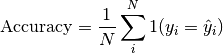
Class Metrics (Classification)¶

Accuracy¶

class pytorch_lightning.metrics.classification.Accuracy(threshold=0.5, top_k=None, subset_accuracy=False, compute_on_step=True, dist_sync_on_step=False, process_group=None, dist_sync_fn=None)[source]

Bases: torchmetrics.

Computes Accuracy:

$\text{Accuracy} = \frac{1}{N}\sum_i^N 1(y_i = \hat{y}_i)$

Where $y$ is a tensor of target values, and $\hat{y}$ is a tensor of predictions.

For multi-class and multi-dimensional multi-class data with probability predictions, the parameter top_k generalizes this metric to a Top-K accuracy metric: for each sample the top-K highest probability items are considered to find the correct label.

For multi-label and multi-dimensional multi-class inputs, this metric computes the “global” accuracy by default, which counts all labels or sub-samples separately. This can be changed to subset accuracy (which requires all labels or sub-samples in the sample to be correctly predicted) by setting subset_accuracy=True.

Accepts all input types listed in Input types.

Parameters

threshold¶ (float) – Threshold probability value for transforming probability predictions to binary (0,1) predictions, in the case of binary or multi-label inputs.
top_k¶ (Optional[int]) –
Number of highest probability predictions considered to find the correct label, relevant only for (multi-dimensional) multi-class inputs with probability predictions. The default value (None) will be interpreted as 1 for these inputs.

Should be left at default (None) for all other types of inputs.
subset_accuracy¶ (bool) –
Whether to compute subset accuracy for multi-label and multi-dimensional multi-class inputs (has no effect for other input types).
- For multi-label inputs, if the parameter is set to True, then all labels for each sample must be correctly predicted for the sample to count as correct. If it is set to False, then all labels are counted separately - this is equivalent to flattening inputs beforehand (i.e. preds = preds.flatten() and same for target).
- For multi-dimensional multi-class inputs, if the parameter is set to True, then all sub-sample (on the extra axis) must be correct for the sample to be counted as correct. If it is set to False, then all sub-samples are counter separately - this is equivalent, in the case of label predictions, to flattening the inputs beforehand (i.e. preds = preds.flatten() and same for target). Note that the top_k parameter still applies in both cases, if set.
compute_on_step¶ (bool) – Forward only calls update() and return None if this is set to False.
dist_sync_on_step¶ (bool) – Synchronize metric state across processes at each forward() before returning the value at the step
process_group¶ (Optional[Any]) – Specify the process group on which synchronization is called. default: None (which selects the entire world)
dist_sync_fn¶ (Optional[Callable]) – Callback that performs the allgather operation on the metric state. When None, DDP will be used to perform the allgather

Example

>>> from pytorch_lightning.metrics import Accuracy
>>> target = torch.tensor([0, 1, 2, 3])
>>> preds = torch.tensor([0, 2, 1, 3])
>>> accuracy = Accuracy()
>>> accuracy(preds, target)
tensor(0.5000)

>>> target = torch.tensor([0, 1, 2])
>>> preds = torch.tensor([[0.1, 0.9, 0], [0.3, 0.1, 0.6], [0.2, 0.5, 0.3]])
>>> accuracy = Accuracy(top_k=2)
>>> accuracy(preds, target)
tensor(0.6667)

compute()[source]

Computes accuracy based on inputs passed in to update previously.

Return type: Tensor

update(preds, target)[source]

Update state with predictions and targets. See Input types for more information on input types.

Parameters

preds¶ (Tensor) – Predictions from model (probabilities, or labels)
target¶ (Tensor) – Ground truth labels

AveragePrecision¶

class pytorch_lightning.metrics.classification.AveragePrecision(num_classes=None, pos_label=None, compute_on_step=True, dist_sync_on_step=False, process_group=None)[source]

Bases: torchmetrics.

Computes the average precision score, which summarises the precision recall curve into one number. Works for both binary and multiclass problems. In the case of multiclass, the values will be calculated based on a one-vs-the-rest approach.

Forward accepts

preds (float tensor): (N, ...) (binary) or (N, C, ...) (multiclass) tensor with probabilities, where C is the number of classes.
target (long tensor): (N, ...) with integer labels

Parameters

num_classes¶ (Optional[int]) – integer with number of classes. Not nessesary to provide for binary problems.
pos_label¶ (Optional[int]) – integer determining the positive class. Default is None which for binary problem is translate to 1. For multiclass problems this argument should not be set as we iteratively change it in the range [0,num_classes-1]
compute_on_step¶ (bool) – Forward only calls update() and return None if this is set to False. default: True
dist_sync_on_step¶ (bool) – Synchronize metric state across processes at each forward() before returning the value at the step. default: False
process_group¶ (Optional[Any]) – Specify the process group on which synchronization is called. default: None (which selects the entire world)

Example (binary case):

>>> pred = torch.tensor([0, 1, 2, 3])
>>> target = torch.tensor([0, 1, 1, 1])
>>> average_precision = AveragePrecision(pos_label=1)
>>> average_precision(pred, target)
tensor(1.)

Example (multiclass case):

>>> pred = torch.tensor([[0.75, 0.05, 0.05, 0.05, 0.05],
...                      [0.05, 0.75, 0.05, 0.05, 0.05],
...                      [0.05, 0.05, 0.75, 0.05, 0.05],
...                      [0.05, 0.05, 0.05, 0.75, 0.05]])
>>> target = torch.tensor([0, 1, 3, 2])
>>> average_precision = AveragePrecision(num_classes=5)
>>> average_precision(pred, target)
[tensor(1.), tensor(1.), tensor(0.2500), tensor(0.2500), tensor(nan)]

compute()[source]

Compute the average precision score

Return type: Union[Tensor, List[Tensor]]
Returns: tensor with average precision. If multiclass will return list of such tensors, one for each class

update(preds, target)[source]

Update state with predictions and targets.

Parameters

preds¶ (Tensor) – Predictions from model
target¶ (Tensor) – Ground truth values

AUC¶

class pytorch_lightning.metrics.classification.AUC(reorder=False, compute_on_step=True, dist_sync_on_step=False, process_group=None, dist_sync_fn=None)[source]

Bases: torchmetrics.

Computes Area Under the Curve (AUC) using the trapezoidal rule

Forward accepts two input tensors that should be 1D and have the same number of elements

Parameters

reorder¶ (bool) – AUC expects its first input to be sorted. If this is not the case, setting this argument to True will use a stable sorting algorithm to sort the input in decending order
compute_on_step¶ (bool) – Forward only calls update() and return None if this is set to False.
dist_sync_on_step¶ (bool) – Synchronize metric state across processes at each forward() before returning the value at the step.
process_group¶ (Optional[Any]) – Specify the process group on which synchronization is called. default: None (which selects the entire world)
dist_sync_fn¶ (Optional[Callable]) – Callback that performs the allgather operation on the metric state. When None, DDP will be used to perform the allgather

compute()[source]

Computes AUC based on inputs passed in to update previously.

Return type: Tensor

update(x, y)[source]

Update state with predictions and targets.

Parameters

x¶ (Tensor) – Predictions from model (probabilities, or labels)
y¶ (Tensor) – Ground truth labels

AUROC¶

class pytorch_lightning.metrics.classification.AUROC(num_classes=None, pos_label=None, average='macro', max_fpr=None, compute_on_step=True, dist_sync_on_step=False, process_group=None, dist_sync_fn=None)[source]

Bases: torchmetrics.

Compute Area Under the Receiver Operating Characteristic Curve (ROC AUC) <https://en.wikipedia.org/wiki/Receiver_operating_characteristic#Further_interpretations>`_. Works for both binary, multilabel and multiclass problems. In the case of multiclass, the values will be calculated based on a one-vs-the-rest approach.

Forward accepts

preds (float tensor): (N, ...) (binary) or (N, C, ...) (multiclass) tensor with probabilities, where C is the number of classes.
target (long tensor): (N, ...) or (N, C, ...) with integer labels

For non-binary input, if the preds and target tensor have the same size the input will be interpretated as multilabel and if preds have one dimension more than the target tensor the input will be interpretated as multiclass.

Args:

num_classes: integer with number of classes. Not nessesary to provide
for binary problems.

pos_label: integer determining the positive class. Default is None
which for binary problem is translate to 1. For multiclass problems this argument should not be set as we iteratively change it in the range [0,num_classes-1]

average:

'macro' computes metric for each class and uniformly averages them

'weighted' computes metric for each class and does a weighted-average, where each class is weighted by their support (accounts for class imbalance)

None computes and returns the metric per class

max_fpr:
If not None, calculates standardized partial AUC over the range [0, max_fpr]. Should be a float between 0 and 1.

compute_on_step:
Forward only calls update() and return None if this is set to False. default: True

dist_sync_on_step:
Synchronize metric state across processes at each forward() before returning the value at the step.

process_group:
Specify the process group on which synchronization is called. default: None (which selects the entire world)

dist_sync_fn:
Callback that performs the allgather operation on the metric state. When None, DDP will be used to perform the allgather

Example (binary case):

>>> preds = torch.tensor([0.13, 0.26, 0.08, 0.19, 0.34])
>>> target = torch.tensor([0, 0, 1, 1, 1])
>>> auroc = AUROC(pos_label=1)
>>> auroc(preds, target)
tensor(0.5000)

Example (multiclass case):

>>> preds = torch.tensor([[0.90, 0.05, 0.05],
...                       [0.05, 0.90, 0.05],
...                       [0.05, 0.05, 0.90],
...                       [0.85, 0.05, 0.10],
...                       [0.10, 0.10, 0.80]])
>>> target = torch.tensor([0, 1, 1, 2, 2])
>>> auroc = AUROC(num_classes=3)
>>> auroc(preds, target)
tensor(0.7778)

compute()[source]

Computes AUROC based on inputs passed in to update previously.

Return type: Tensor

update(preds, target)[source]

Update state with predictions and targets.

Parameters

preds¶ (Tensor) – Predictions from model (probabilities, or labels)
target¶ (Tensor) – Ground truth labels

ConfusionMatrix¶

class pytorch_lightning.metrics.classification.ConfusionMatrix(num_classes, normalize=None, threshold=0.5, compute_on_step=True, dist_sync_on_step=False, process_group=None)[source]

Bases: torchmetrics.

Computes the confusion matrix. Works with binary, multiclass, and multilabel data. Accepts probabilities from a model output or integer class values in prediction. Works with multi-dimensional preds and target.

Note

This metric produces a multi-dimensional output, so it can not be directly logged.

Forward accepts

preds (float or long tensor): (N, ...) or (N, C, ...) where C is the number of classes
target (long tensor): (N, ...)

If preds and target are the same shape and preds is a float tensor, we use the self.threshold argument to convert into integer labels. This is the case for binary and multi-label probabilities.

If preds has an extra dimension as in the case of multi-class scores we perform an argmax on dim=1.

Parameters

num_classes¶ (int) – Number of classes in the dataset.
normalize¶ (Optional[str]) –
Normalization mode for confusion matrix. Choose from
- None or 'none': no normalization (default)
- 'true': normalization over the targets (most commonly used)
- 'pred': normalization over the predictions
- 'all': normalization over the whole matrix
threshold¶ (float) – Threshold value for binary or multi-label probabilites. default: 0.5
compute_on_step¶ (bool) – Forward only calls update() and return None if this is set to False. default: True
dist_sync_on_step¶ (bool) – Synchronize metric state across processes at each forward() before returning the value at the step. default: False
process_group¶ (Optional[Any]) – Specify the process group on which synchronization is called. default: None (which selects the entire world)

Example

>>> from pytorch_lightning.metrics import ConfusionMatrix
>>> target = torch.tensor([1, 1, 0, 0])
>>> preds = torch.tensor([0, 1, 0, 0])
>>> confmat = ConfusionMatrix(num_classes=2)
>>> confmat(preds, target)
tensor([[2., 0.],
        [1., 1.]])

compute()[source]

Computes confusion matrix

Return type: Tensor

update(preds, target)[source]

Update state with predictions and targets.

Parameters

preds¶ (Tensor) – Predictions from model
target¶ (Tensor) – Ground truth values

F1¶

class pytorch_lightning.metrics.classification.F1(num_classes, threshold=0.5, average='micro', multilabel=False, compute_on_step=True, dist_sync_on_step=False, process_group=None)[source]

Bases: torchmetrics.

Computes F1 metric. F1 metrics correspond to a harmonic mean of the precision and recall scores.

Works with binary, multiclass, and multilabel data. Accepts logits from a model output or integer class values in prediction. Works with multi-dimensional preds and target.

Forward accepts

preds (float or long tensor): (N, ...) or (N, C, ...) where C is the number of classes
target (long tensor): (N, ...)

If preds and target are the same shape and preds is a float tensor, we use the self.threshold argument. This is the case for binary and multi-label logits.

If preds has an extra dimension as in the case of multi-class scores we perform an argmax on dim=1.

Parameters

num_classes¶ (int) – Number of classes in the dataset.
threshold¶ (float) – Threshold value for binary or multi-label logits. default: 0.5
average¶ (str) –
- 'micro' computes metric globally
- 'macro' computes metric for each class and uniformly averages them
- 'weighted' computes metric for each class and does a weighted-average, where each class is weighted by their support (accounts for class imbalance)
- 'none' or None computes and returns the metric per class
multilabel¶ (bool) – If predictions are from multilabel classification.
compute_on_step¶ (bool) – Forward only calls update() and returns None if this is set to False. default: True
dist_sync_on_step¶ (bool) – Synchronize metric state across processes at each forward() before returning the value at the step. default: False
process_group¶ (Optional[Any]) – Specify the process group on which synchronization is called. default: None (which selects the entire world)

Example

>>> from pytorch_lightning.metrics import F1
>>> target = torch.tensor([0, 1, 2, 0, 1, 2])
>>> preds = torch.tensor([0, 2, 1, 0, 0, 1])
>>> f1 = F1(num_classes=3)
>>> f1(preds, target)
tensor(0.3333)

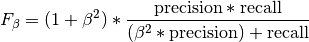
FBeta¶

class pytorch_lightning.metrics.classification.FBeta(num_classes, beta=1.0, threshold=0.5, average='micro', multilabel=False, compute_on_step=True, dist_sync_on_step=False, process_group=None)[source]

Bases: torchmetrics.

Computes F-score, specifically:

$F_\beta = (1 + \beta^2) * \frac{\text{precision} * \text{recall}} {(\beta^2 * \text{precision}) + \text{recall}}$

Where $\beta$ is some positive real factor. Works with binary, multiclass, and multilabel data. Accepts probabilities from a model output or integer class values in prediction. Works with multi-dimensional preds and target.

Forward accepts

preds (float or long tensor): (N, ...) or (N, C, ...) where C is the number of classes
target (long tensor): (N, ...)

If preds and target are the same shape and preds is a float tensor, we use the self.threshold argument to convert into integer labels. This is the case for binary and multi-label probabilities.

If preds has an extra dimension as in the case of multi-class scores we perform an argmax on dim=1.

Parameters

num_classes¶ (int) – Number of classes in the dataset.
beta¶ (float) – Beta coefficient in the F measure.
threshold¶ (float) – Threshold value for binary or multi-label probabilities. default: 0.5
average¶ (str) –
- 'micro' computes metric globally
- 'macro' computes metric for each class and uniformly averages them
- 'weighted' computes metric for each class and does a weighted-average, where each class is weighted by their support (accounts for class imbalance)
- 'none' or None computes and returns the metric per class
multilabel¶ (bool) – If predictions are from multilabel classification.
compute_on_step¶ (bool) – Forward only calls update() and return None if this is set to False. default: True
dist_sync_on_step¶ (bool) – Synchronize metric state across processes at each forward() before returning the value at the step. default: False
process_group¶ (Optional[Any]) – Specify the process group on which synchronization is called. default: None (which selects the entire world)

Example

>>> from pytorch_lightning.metrics import FBeta
>>> target = torch.tensor([0, 1, 2, 0, 1, 2])
>>> preds = torch.tensor([0, 2, 1, 0, 0, 1])
>>> f_beta = FBeta(num_classes=3, beta=0.5)
>>> f_beta(preds, target)
tensor(0.3333)

compute()[source]

Computes fbeta over state.

Return type: Tensor

update(preds, target)[source]

Update state with predictions and targets.

Parameters

preds¶ (Tensor) – Predictions from model
target¶ (Tensor) – Ground truth values

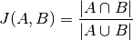
IoU¶

class pytorch_lightning.metrics.classification.IoU(num_classes, ignore_index=None, absent_score=0.0, threshold=0.5, reduction='elementwise_mean', compute_on_step=True, dist_sync_on_step=False, process_group=None)[source]

Bases: torchmetrics.

Computes Intersection over union, or Jaccard index calculation:

$J(A,B) = \frac{|A\cap B|}{|A\cup B|}$

Where: $A$ and $B$ are both tensors of the same size, containing integer class values. They may be subject to conversion from input data (see description below). Note that it is different from box IoU.

Works with binary, multiclass and multi-label data. Accepts probabilities from a model output or integer class values in prediction. Works with multi-dimensional preds and target.

Forward accepts

preds (float or long tensor): (N, ...) or (N, C, ...) where C is the number of classes
target (long tensor): (N, ...)

If preds and target are the same shape and preds is a float tensor, we use the self.threshold argument to convert into integer labels. This is the case for binary and multi-label probabilities.

If preds has an extra dimension as in the case of multi-class scores we perform an argmax on dim=1.

Parameters

num_classes¶ (int) – Number of classes in the dataset.
ignore_index¶ (Optional[int]) – optional int specifying a target class to ignore. If given, this class index does not contribute to the returned score, regardless of reduction method. Has no effect if given an int that is not in the range [0, num_classes-1]. By default, no index is ignored, and all classes are used.
absent_score¶ (float) – score to use for an individual class, if no instances of the class index were present in pred AND no instances of the class index were present in target. For example, if we have 3 classes, [0, 0] for pred, and [0, 2] for target, then class 1 would be assigned the absent_score.
threshold¶ (float) – Threshold value for binary or multi-label probabilities.
reduction¶ (str) –
a method to reduce metric score over labels.
- 'elementwise_mean': takes the mean (default)
- 'sum': takes the sum
- 'none': no reduction will be applied
compute_on_step¶ (bool) – Forward only calls update() and return None if this is set to False.
dist_sync_on_step¶ (bool) – Synchronize metric state across processes at each forward() before returning the value at the step.
process_group¶ (Optional[Any]) – Specify the process group on which synchronization is called. default: None (which selects the entire world)

Example

>>> from pytorch_lightning.metrics import IoU
>>> target = torch.randint(0, 2, (10, 25, 25))
>>> pred = torch.tensor(target)
>>> pred[2:5, 7:13, 9:15] = 1 - pred[2:5, 7:13, 9:15]
>>> iou = IoU(num_classes=2)
>>> iou(pred, target)
tensor(0.9660)

compute()[source]

Computes intersection over union (IoU)

Return type: Tensor

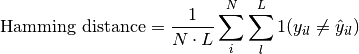
Hamming Distance¶

class pytorch_lightning.metrics.classification.HammingDistance(threshold=0.5, compute_on_step=True, dist_sync_on_step=False, process_group=None, dist_sync_fn=None)[source]

Bases: torchmetrics.

Computes the average Hamming distance (also known as Hamming loss) between targets and predictions:

$\text{Hamming distance} = \frac{1}{N \cdot L}\sum_i^N \sum_l^L 1(y_{il} \neq \hat{y_{il}})$

Where $y$ is a tensor of target values, $\hat{y}$ is a tensor of predictions, and $\bullet_{il}$ refers to the $l$ -th label of the $i$ -th sample of that tensor.

This is the same as 1-accuracy for binary data, while for all other types of inputs it treats each possible label separately - meaning that, for example, multi-class data is treated as if it were multi-label.

Accepts all input types listed in Input types.

Parameters

threshold¶ (float) – Threshold probability value for transforming probability predictions to binary (0 or 1) predictions, in the case of binary or multi-label inputs.
compute_on_step¶ (bool) – Forward only calls update() and return None if this is set to False.
dist_sync_on_step¶ (bool) – Synchronize metric state across processes at each forward() before returning the value at the step.
process_group¶ (Optional[Any]) – Specify the process group on which synchronization is called. default: None (which selects the entire world)
dist_sync_fn¶ (Optional[Callable]) – Callback that performs the allgather operation on the metric state. When None, DDP will be used to perform the all gather.

Example

>>> from pytorch_lightning.metrics import HammingDistance
>>> target = torch.tensor([[0, 1], [1, 1]])
>>> preds = torch.tensor([[0, 1], [0, 1]])
>>> hamming_distance = HammingDistance()
>>> hamming_distance(preds, target)
tensor(0.2500)

compute()[source]

Computes hamming distance based on inputs passed in to update previously.

Return type: Tensor

update(preds, target)[source]

Update state with predictions and targets. See Input types for more information on input types.

Parameters

preds¶ (Tensor) – Predictions from model (probabilities, or labels)
target¶ (Tensor) – Ground truth labels

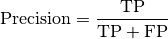
Precision¶

class pytorch_lightning.metrics.classification.Precision(num_classes=None, threshold=0.5, average='micro', multilabel=False, mdmc_average=None, ignore_index=None, top_k=None, is_multiclass=None, compute_on_step=True, dist_sync_on_step=False, process_group=None, dist_sync_fn=None)[source]

Bases: torchmetrics.

Computes Precision:

$\text{Precision} = \frac{\text{TP}}{\text{TP} + \text{FP}}$

Where $\text{TP}$ and $\text{FP}$ represent the number of true positives and false positives respecitively. With the use of top_k parameter, this metric can generalize to Precision@K.

The reduction method (how the precision scores are aggregated) is controlled by the average parameter, and additionally by the mdmc_average parameter in the multi-dimensional multi-class case. Accepts all inputs listed in Input types.

Parameters

num_classes¶ (Optional[int]) – Number of classes. Necessary for 'macro', 'weighted' and None average methods.
threshold¶ (float) – Threshold probability value for transforming probability predictions to binary (0,1) predictions, in the case of binary or multi-label inputs.
average¶ (str) –
Defines the reduction that is applied. Should be one of the following:
- 'micro' [default]: Calculate the metric globally, accross all samples and classes.
- 'macro': Calculate the metric for each class separately, and average the metrics accross classes (with equal weights for each class).
- 'weighted': Calculate the metric for each class separately, and average the metrics accross classes, weighting each class by its support (tp + fn).
- 'none' or None: Calculate the metric for each class separately, and return the metric for every class.
- 'samples': Calculate the metric for each sample, and average the metrics across samples (with equal weights for each sample).
Note that what is considered a sample in the multi-dimensional multi-class case depends on the value of mdmc_average.
multilabel¶ (bool) –

Warning

This parameter is deprecated and has no effect. Will be removed in v1.4.0.
mdmc_average¶ (Optional[str]) –
Defines how averaging is done for multi-dimensional multi-class inputs (on top of the average parameter). Should be one of the following:
- None [default]: Should be left unchanged if your data is not multi-dimensional multi-class.
- 'samplewise': In this case, the statistics are computed separately for each sample on the N axis, and then averaged over samples. The computation for each sample is done by treating the flattened extra axes ... (see Input types) as the N dimension within the sample, and computing the metric for the sample based on that.
- 'global': In this case the N and ... dimensions of the inputs (see Input types) are flattened into a new N_X sample axis, i.e. the inputs are treated as if they were (N_X, C). From here on the average parameter applies as usual.
ignore_index¶ (Optional[int]) – Integer specifying a target class to ignore. If given, this class index does not contribute to the returned score, regardless of reduction method. If an index is ignored, and average=None or 'none', the score for the ignored class will be returned as nan.
top_k¶ (Optional[int]) –
Number of highest probability entries for each sample to convert to 1s - relevant only for inputs with probability predictions. If this parameter is set for multi-label inputs, it will take precedence over threshold. For (multi-dim) multi-class inputs, this parameter defaults to 1.

Should be left unset (None) for inputs with label predictions.
is_multiclass¶ (Optional[bool]) – Used only in certain special cases, where you want to treat inputs as a different type than what they appear to be. See the parameter’s documentation section for a more detailed explanation and examples.
compute_on_step¶ (bool) – Forward only calls update() and return None if this is set to False.
dist_sync_on_step¶ (bool) – Synchronize metric state across processes at each forward() before returning the value at the step
process_group¶ (Optional[Any]) – Specify the process group on which synchronization is called. default: None (which selects the entire world)
dist_sync_fn¶ (Optional[Callable]) – Callback that performs the allgather operation on the metric state. When None, DDP will be used to perform the allgather.

Example

>>> from pytorch_lightning.metrics import Precision
>>> preds  = torch.tensor([2, 0, 2, 1])
>>> target = torch.tensor([1, 1, 2, 0])
>>> precision = Precision(average='macro', num_classes=3)
>>> precision(preds, target)
tensor(0.1667)
>>> precision = Precision(average='micro')
>>> precision(preds, target)
tensor(0.2500)

compute()[source]

Computes the precision score based on inputs passed in to update previously.

Return type

Tensor

Returns

The shape of the returned tensor depends on the average parameter

If average in ['micro', 'macro', 'weighted', 'samples'], a one-element tensor will be returned
If average in ['none', None], the shape will be (C,), where C stands for the number of classes

PrecisionRecallCurve¶

class pytorch_lightning.metrics.classification.PrecisionRecallCurve(num_classes=None, pos_label=None, compute_on_step=True, dist_sync_on_step=False, process_group=None)[source]

Bases: torchmetrics.

Computes precision-recall pairs for different thresholds. Works for both binary and multiclass problems. In the case of multiclass, the values will be calculated based on a one-vs-the-rest approach.

Forward accepts

preds (float tensor): (N, ...) (binary) or (N, C, ...) (multiclass) tensor with probabilities, where C is the number of classes.
target (long tensor): (N, ...) or (N, C, ...) with integer labels

Parameters

num_classes¶ (Optional[int]) – integer with number of classes. Not nessesary to provide for binary problems.
pos_label¶ (Optional[int]) – integer determining the positive class. Default is None which for binary problem is translate to 1. For multiclass problems this argument should not be set as we iteratively change it in the range [0,num_classes-1]
compute_on_step¶ (bool) – Forward only calls update() and return None if this is set to False. default: True
dist_sync_on_step¶ (bool) – Synchronize metric state across processes at each forward() before returning the value at the step. default: False
process_group¶ (Optional[Any]) – Specify the process group on which synchronization is called. default: None (which selects the entire world)

Example (binary case):

>>> pred = torch.tensor([0, 1, 2, 3])
>>> target = torch.tensor([0, 1, 1, 0])
>>> pr_curve = PrecisionRecallCurve(pos_label=1)
>>> precision, recall, thresholds = pr_curve(pred, target)
>>> precision
tensor([0.6667, 0.5000, 0.0000, 1.0000])
>>> recall
tensor([1.0000, 0.5000, 0.0000, 0.0000])
>>> thresholds
tensor([1, 2, 3])

Example (multiclass case):

>>> pred = torch.tensor([[0.75, 0.05, 0.05, 0.05, 0.05],
...                      [0.05, 0.75, 0.05, 0.05, 0.05],
...                      [0.05, 0.05, 0.75, 0.05, 0.05],
...                      [0.05, 0.05, 0.05, 0.75, 0.05]])
>>> target = torch.tensor([0, 1, 3, 2])
>>> pr_curve = PrecisionRecallCurve(num_classes=5)
>>> precision, recall, thresholds = pr_curve(pred, target)
>>> precision   
[tensor([1., 1.]), tensor([1., 1.]), tensor([0.2500, 0.0000, 1.0000]),
 tensor([0.2500, 0.0000, 1.0000]), tensor([0., 1.])]
>>> recall
[tensor([1., 0.]), tensor([1., 0.]), tensor([1., 0., 0.]), tensor([1., 0., 0.]), tensor([nan, 0.])]
>>> thresholds
[tensor([0.7500]), tensor([0.7500]), tensor([0.0500, 0.7500]), tensor([0.0500, 0.7500]), tensor([0.0500])]

compute()[source]

Compute the precision-recall curve

Returns: 3-element tuple containing

precision:
tensor where element i is the precision of predictions with score >= thresholds[i] and the last element is 1. If multiclass, this is a list of such tensors, one for each class.

recall:
tensor where element i is the recall of predictions with score >= thresholds[i] and the last element is 0. If multiclass, this is a list of such tensors, one for each class.

thresholds:
Thresholds used for computing precision/recall scores

Return type: Union[Tuple[Tensor, Tensor, Tensor], Tuple[List[Tensor], List[Tensor], List[Tensor]]]

update(preds, target)[source]

Update state with predictions and targets.

Parameters

preds¶ (Tensor) – Predictions from model
target¶ (Tensor) – Ground truth values

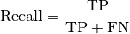
Recall¶

class pytorch_lightning.metrics.classification.Recall(num_classes=None, threshold=0.5, average='micro', multilabel=False, mdmc_average=None, ignore_index=None, top_k=None, is_multiclass=None, compute_on_step=True, dist_sync_on_step=False, process_group=None, dist_sync_fn=None)[source]

Bases: torchmetrics.

Computes Recall:

$\text{Recall} = \frac{\text{TP}}{\text{TP} + \text{FN}}$

Where $\text{TP}$ and $\text{FN}$ represent the number of true positives and false negatives respecitively. With the use of top_k parameter, this metric can generalize to Recall@K.

The reduction method (how the recall scores are aggregated) is controlled by the average parameter, and additionally by the mdmc_average parameter in the multi-dimensional multi-class case. Accepts all inputs listed in Input types.

Parameters

num_classes¶ (Optional[int]) – Number of classes. Necessary for 'macro', 'weighted' and None average methods.
threshold¶ (float) – Threshold probability value for transforming probability predictions to binary (0,1) predictions, in the case of binary or multi-label inputs.
average¶ (str) –
Defines the reduction that is applied. Should be one of the following:
- 'micro' [default]: Calculate the metric globally, accross all samples and classes.
- 'macro': Calculate the metric for each class separately, and average the metrics accross classes (with equal weights for each class).
- 'weighted': Calculate the metric for each class separately, and average the metrics accross classes, weighting each class by its support (tp + fn).
- 'none' or None: Calculate the metric for each class separately, and return the metric for every class.
- 'samples': Calculate the metric for each sample, and average the metrics across samples (with equal weights for each sample).
Note that what is considered a sample in the multi-dimensional multi-class case depends on the value of mdmc_average.
multilabel¶ (bool) –

Warning

This parameter is deprecated and has no effect. Will be removed in v1.4.0.
mdmc_average¶ (Optional[str]) –
Defines how averaging is done for multi-dimensional multi-class inputs (on top of the average parameter). Should be one of the following:
- None [default]: Should be left unchanged if your data is not multi-dimensional multi-class.
- 'samplewise': In this case, the statistics are computed separately for each sample on the N axis, and then averaged over samples. The computation for each sample is done by treating the flattened extra axes ... (see Input types) as the N dimension within the sample, and computing the metric for the sample based on that.
- 'global': In this case the N and ... dimensions of the inputs (see Input types) are flattened into a new N_X sample axis, i.e. the inputs are treated as if they were (N_X, C). From here on the average parameter applies as usual.
ignore_index¶ (Optional[int]) – Integer specifying a target class to ignore. If given, this class index does not contribute to the returned score, regardless of reduction method. If an index is ignored, and average=None or 'none', the score for the ignored class will be returned as nan.
top_k¶ (Optional[int]) –
Number of highest probability entries for each sample to convert to 1s - relevant only for inputs with probability predictions. If this parameter is set for multi-label inputs, it will take precedence over threshold. For (multi-dim) multi-class inputs, this parameter defaults to 1.

Should be left unset (None) for inputs with label predictions.
is_multiclass¶ (Optional[bool]) – Used only in certain special cases, where you want to treat inputs as a different type than what they appear to be. See the parameter’s documentation section for a more detailed explanation and examples.
compute_on_step¶ (bool) – Forward only calls update() and return None if this is set to False.
dist_sync_on_step¶ (bool) – Synchronize metric state across processes at each forward() before returning the value at the step
process_group¶ (Optional[Any]) – Specify the process group on which synchronization is called. default: None (which selects the entire world)
dist_sync_fn¶ (Optional[Callable]) – Callback that performs the allgather operation on the metric state. When None, DDP will be used to perform the allgather.

Example

>>> from pytorch_lightning.metrics import Recall
>>> preds  = torch.tensor([2, 0, 2, 1])
>>> target = torch.tensor([1, 1, 2, 0])
>>> recall = Recall(average='macro', num_classes=3)
>>> recall(preds, target)
tensor(0.3333)
>>> recall = Recall(average='micro')
>>> recall(preds, target)
tensor(0.2500)

compute()[source]

Computes the recall score based on inputs passed in to update previously.

Return type

Tensor

Returns

The shape of the returned tensor depends on the average parameter

If average in ['micro', 'macro', 'weighted', 'samples'], a one-element tensor will be returned
If average in ['none', None], the shape will be (C,), where C stands for the number of classes

ROC¶

class pytorch_lightning.metrics.classification.ROC(num_classes=None, pos_label=None, compute_on_step=True, dist_sync_on_step=False, process_group=None)[source]

Bases: torchmetrics.

Computes the Receiver Operating Characteristic (ROC). Works for both binary and multiclass problems. In the case of multiclass, the values will be calculated based on a one-vs-the-rest approach.

Forward accepts

preds (float tensor): (N, ...) (binary) or (N, C, ...) (multiclass) tensor with probabilities, where C is the number of classes.
target (long tensor): (N, ...) or (N, C, ...) with integer labels

Parameters

num_classes¶ (Optional[int]) – integer with number of classes. Not nessesary to provide for binary problems.
pos_label¶ (Optional[int]) – integer determining the positive class. Default is None which for binary problem is translate to 1. For multiclass problems this argument should not be set as we iteratively change it in the range [0,num_classes-1]
compute_on_step¶ (bool) – Forward only calls update() and return None if this is set to False. default: True
dist_sync_on_step¶ (bool) – Synchronize metric state across processes at each forward() before returning the value at the step. default: False
process_group¶ (Optional[Any]) – Specify the process group on which synchronization is called. default: None (which selects the entire world)

Example (binary case):

>>> pred = torch.tensor([0, 1, 2, 3])
>>> target = torch.tensor([0, 1, 1, 1])
>>> roc = ROC(pos_label=1)
>>> fpr, tpr, thresholds = roc(pred, target)
>>> fpr
tensor([0., 0., 0., 0., 1.])
>>> tpr
tensor([0.0000, 0.3333, 0.6667, 1.0000, 1.0000])
>>> thresholds
tensor([4, 3, 2, 1, 0])

Example (multiclass case):

>>> pred = torch.tensor([[0.75, 0.05, 0.05, 0.05],
...                      [0.05, 0.75, 0.05, 0.05],
...                      [0.05, 0.05, 0.75, 0.05],
...                      [0.05, 0.05, 0.05, 0.75]])
>>> target = torch.tensor([0, 1, 3, 2])
>>> roc = ROC(num_classes=4)
>>> fpr, tpr, thresholds = roc(pred, target)
>>> fpr
[tensor([0., 0., 1.]), tensor([0., 0., 1.]), tensor([0.0000, 0.3333, 1.0000]), tensor([0.0000, 0.3333, 1.0000])]
>>> tpr
[tensor([0., 1., 1.]), tensor([0., 1., 1.]), tensor([0., 0., 1.]), tensor([0., 0., 1.])]
>>> thresholds 
[tensor([1.7500, 0.7500, 0.0500]),
 tensor([1.7500, 0.7500, 0.0500]),
 tensor([1.7500, 0.7500, 0.0500]),
 tensor([1.7500, 0.7500, 0.0500])]

compute()[source]

Compute the receiver operating characteristic

Returns: 3-element tuple containing

fpr:
tensor with false positive rates. If multiclass, this is a list of such tensors, one for each class.

tpr:
tensor with true positive rates. If multiclass, this is a list of such tensors, one for each class.

thresholds:
thresholds used for computing false- and true postive rates

Return type: Union[Tuple[Tensor, Tensor, Tensor], Tuple[List[Tensor], List[Tensor], List[Tensor]]]

update(preds, target)[source]

Update state with predictions and targets.

Parameters

preds¶ (Tensor) – Predictions from model
target¶ (Tensor) – Ground truth values

StatScores¶

class pytorch_lightning.metrics.classification.StatScores(threshold=0.5, top_k=None, reduce='micro', num_classes=None, ignore_index=None, mdmc_reduce=None, is_multiclass=None, compute_on_step=True, dist_sync_on_step=False, process_group=None, dist_sync_fn=None)[source]

Bases: torchmetrics.

Computes the number of true positives, false positives, true negatives, false negatives. Related to Type I and Type II errors and the confusion matrix.

The reduction method (how the statistics are aggregated) is controlled by the reduce parameter, and additionally by the mdmc_reduce parameter in the multi-dimensional multi-class case.

Accepts all inputs listed in Input types.

Parameters

threshold¶ (float) – Threshold probability value for transforming probability predictions to binary (0 or 1) predictions, in the case of binary or multi-label inputs.
top_k¶ (Optional[int]) –
Number of highest probability entries for each sample to convert to 1s - relevant only for inputs with probability predictions. If this parameter is set for multi-label inputs, it will take precedence over threshold. For (multi-dim) multi-class inputs, this parameter defaults to 1.

Should be left unset (None) for inputs with label predictions.
reduce¶ (str) –
Defines the reduction that is applied. Should be one of the following:
- 'micro' [default]: Counts the statistics by summing over all [sample, class] combinations (globally). Each statistic is represented by a single integer.
- 'macro': Counts the statistics for each class separately (over all samples). Each statistic is represented by a (C,) tensor. Requires num_classes to be set.
- 'samples': Counts the statistics for each sample separately (over all classes). Each statistic is represented by a (N, ) 1d tensor.
Note that what is considered a sample in the multi-dimensional multi-class case depends on the value of mdmc_reduce.
num_classes¶ (Optional[int]) – Number of classes. Necessary for (multi-dimensional) multi-class or multi-label data.
ignore_index¶ (Optional[int]) – Specify a class (label) to ignore. If given, this class index does not contribute to the returned score, regardless of reduction method. If an index is ignored, and reduce='macro', the class statistics for the ignored class will all be returned as -1.
mdmc_reduce¶ (Optional[str]) –
Defines how the multi-dimensional multi-class inputs are handeled. Should be one of the following:
- None [default]: Should be left unchanged if your data is not multi-dimensional multi-class (see Input types for the definition of input types).
- 'samplewise': In this case, the statistics are computed separately for each sample on the N axis, and then the outputs are concatenated together. In each sample the extra axes ... are flattened to become the sub-sample axis, and statistics for each sample are computed by treating the sub-sample axis as the N axis for that sample.
- 'global': In this case the N and ... dimensions of the inputs are flattened into a new N_X sample axis, i.e. the inputs are treated as if they were (N_X, C). From here on the reduce parameter applies as usual.
is_multiclass¶ (Optional[bool]) – Used only in certain special cases, where you want to treat inputs as a different type than what they appear to be. See the parameter’s documentation section for a more detailed explanation and examples.
compute_on_step¶ (bool) – Forward only calls update() and return None if this is set to False.
dist_sync_on_step¶ (bool) – Synchronize metric state across processes at each forward() before returning the value at the step
process_group¶ (Optional[Any]) – Specify the process group on which synchronization is called. default: None (which selects the entire world)
dist_sync_fn¶ (Optional[Callable]) – Callback that performs the allgather operation on the metric state. When None, DDP will be used to perform the allgather.

Example

>>> from pytorch_lightning.metrics.classification import StatScores
>>> preds  = torch.tensor([1, 0, 2, 1])
>>> target = torch.tensor([1, 1, 2, 0])
>>> stat_scores = StatScores(reduce='macro', num_classes=3)
>>> stat_scores(preds, target)
tensor([[0, 1, 2, 1, 1],
        [1, 1, 1, 1, 2],
        [1, 0, 3, 0, 1]])
>>> stat_scores = StatScores(reduce='micro')
>>> stat_scores(preds, target)
tensor([2, 2, 6, 2, 4])

compute()[source]

Computes the stat scores based on inputs passed in to update previously.

Return type

Tensor

Returns

The metric returns a tensor of shape (..., 5), where the last dimension corresponds to [tp, fp, tn, fn, sup] (sup stands for support and equals tp + fn). The shape depends on the reduce and mdmc_reduce (in case of multi-dimensional multi-class data) parameters:

If the data is not multi-dimensional multi-class, then
- If reduce='micro', the shape will be (5, )
- If reduce='macro', the shape will be (C, 5), where C stands for the number of classes
- If reduce='samples', the shape will be (N, 5), where N stands for the number of samples
If the data is multi-dimensional multi-class and mdmc_reduce='global', then
- If reduce='micro', the shape will be (5, )
- If reduce='macro', the shape will be (C, 5)
- If reduce='samples', the shape will be (N*X, 5), where X stands for the product of sizes of all “extra” dimensions of the data (i.e. all dimensions except for C and N)
If the data is multi-dimensional multi-class and mdmc_reduce='samplewise', then
- If reduce='micro', the shape will be (N, 5)
- If reduce='macro', the shape will be (N, C, 5)
- If reduce='samples', the shape will be (N, X, 5)

update(preds, target)[source]

Update state with predictions and targets. See Input types for more information on input types.

Parameters

preds¶ (Tensor) – Predictions from model (probabilities or labels)
target¶ (Tensor) – Ground truth values

Functional Metrics (Classification)¶

accuracy [func]¶

pytorch_lightning.metrics.functional.accuracy(preds, target, threshold=0.5, top_k=None, subset_accuracy=False)[source]

Computes Accuracy:

$\text{Accuracy} = \frac{1}{N}\sum_i^N 1(y_i = \hat{y}_i)$

Where $y$ is a tensor of target values, and $\hat{y}$ is a tensor of predictions.

For multi-class and multi-dimensional multi-class data with probability predictions, the parameter top_k generalizes this metric to a Top-K accuracy metric: for each sample the top-K highest probability items are considered to find the correct label.

For multi-label and multi-dimensional multi-class inputs, this metric computes the “global” accuracy by default, which counts all labels or sub-samples separately. This can be changed to subset accuracy (which requires all labels or sub-samples in the sample to be correctly predicted) by setting subset_accuracy=True.

Accepts all input types listed in Input types.

Parameters

preds¶ (Tensor) – Predictions from model (probabilities, or labels)
target¶ (Tensor) – Ground truth labels
threshold¶ (float) – Threshold probability value for transforming probability predictions to binary (0,1) predictions, in the case of binary or multi-label inputs.
top_k¶ (Optional[int]) –
Number of highest probability predictions considered to find the correct label, relevant only for (multi-dimensional) multi-class inputs with probability predictions. The default value (None) will be interpreted as 1 for these inputs.

Should be left at default (None) for all other types of inputs.
subset_accuracy¶ (bool) –
Whether to compute subset accuracy for multi-label and multi-dimensional multi-class inputs (has no effect for other input types).
- For multi-label inputs, if the parameter is set to True, then all labels for each sample must be correctly predicted for the sample to count as correct. If it is set to False, then all labels are counted separately - this is equivalent to flattening inputs beforehand (i.e. preds = preds.flatten() and same for target).
- For multi-dimensional multi-class inputs, if the parameter is set to True, then all sub-sample (on the extra axis) must be correct for the sample to be counted as correct. If it is set to False, then all sub-samples are counter separately - this is equivalent, in the case of label predictions, to flattening the inputs beforehand (i.e. preds = preds.flatten() and same for target). Note that the top_k parameter still applies in both cases, if set.

Example

>>> from pytorch_lightning.metrics.functional import accuracy
>>> target = torch.tensor([0, 1, 2, 3])
>>> preds = torch.tensor([0, 2, 1, 3])
>>> accuracy(preds, target)
tensor(0.5000)

>>> target = torch.tensor([0, 1, 2])
>>> preds = torch.tensor([[0.1, 0.9, 0], [0.3, 0.1, 0.6], [0.2, 0.5, 0.3]])
>>> accuracy(preds, target, top_k=2)
tensor(0.6667)

Return type: Tensor

auc [func]¶

pytorch_lightning.metrics.functional.auc(x, y, reorder=False)[source]

Computes Area Under the Curve (AUC) using the trapezoidal rule

Parameters

x¶ (Tensor) – x-coordinates
y¶ (Tensor) – y-coordinates
reorder¶ (bool) – if True, will reorder the arrays

Return type

Tensor

Returns

Tensor containing AUC score (float)

Example

>>> x = torch.tensor([0, 1, 2, 3])
>>> y = torch.tensor([0, 1, 2, 2])
>>> auc(x, y)
tensor(4.)

auroc [func]¶

pytorch_lightning.metrics.functional.auroc(preds, target, num_classes=None, pos_label=None, average='macro', max_fpr=None, sample_weights=None)[source]

Compute Area Under the Receiver Operating Characteristic Curve (ROC AUC)

Parameters

preds¶ (Tensor) – predictions from model (logits or probabilities)
target¶ (Tensor) – Ground truth labels
num_classes¶ (Optional[int]) – integer with number of classes. Not nessesary to provide for binary problems.
pos_label¶ (Optional[int]) – integer determining the positive class. Default is None which for binary problem is translate to 1. For multiclass problems this argument should not be set as we iteratively change it in the range [0,num_classes-1]
average¶ (Optional[str]) –
- 'macro' computes metric for each class and uniformly averages them
- 'weighted' computes metric for each class and does a weighted-average, where each class is weighted by their support (accounts for class imbalance)
- None computes and returns the metric per class
max_fpr¶ (Optional[float]) – If not None, calculates standardized partial AUC over the range [0, max_fpr]. Should be a float between 0 and 1.
sample_weight¶ – sample weights for each data point

Example (binary case):

>>> preds = torch.tensor([0.13, 0.26, 0.08, 0.19, 0.34])
>>> target = torch.tensor([0, 0, 1, 1, 1])
>>> auroc(preds, target, pos_label=1)
tensor(0.5000)

Example (multiclass case):

>>> preds = torch.tensor([[0.90, 0.05, 0.05],
...                       [0.05, 0.90, 0.05],
...                       [0.05, 0.05, 0.90],
...                       [0.85, 0.05, 0.10],
...                       [0.10, 0.10, 0.80]])
>>> target = torch.tensor([0, 1, 1, 2, 2])
>>> auroc(preds, target, num_classes=3)
tensor(0.7778)

Return type: Tensor

average_precision [func]¶

pytorch_lightning.metrics.functional.average_precision(preds, target, num_classes=None, pos_label=None, sample_weights=None)[source]

Computes the average precision score.

Parameters

preds¶ (Tensor) – predictions from model (logits or probabilities)
target¶ (Tensor) – ground truth values
num_classes¶ (Optional[int]) – integer with number of classes. Not nessesary to provide for binary problems.
pos_label¶ (Optional[int]) – integer determining the positive class. Default is None which for binary problem is translate to 1. For multiclass problems this argument should not be set as we iteratively change it in the range [0,num_classes-1]
sample_weights¶ (Optional[Sequence]) – sample weights for each data point

Return type

Union[List[Tensor], Tensor]

Returns

tensor with average precision. If multiclass will return list of such tensors, one for each class

Example (binary case):

>>> pred = torch.tensor([0, 1, 2, 3])
>>> target = torch.tensor([0, 1, 1, 1])
>>> average_precision(pred, target, pos_label=1)
tensor(1.)

Example (multiclass case):

>>> pred = torch.tensor([[0.75, 0.05, 0.05, 0.05, 0.05],
...                      [0.05, 0.75, 0.05, 0.05, 0.05],
...                      [0.05, 0.05, 0.75, 0.05, 0.05],
...                      [0.05, 0.05, 0.05, 0.75, 0.05]])
>>> target = torch.tensor([0, 1, 3, 2])
>>> average_precision(pred, target, num_classes=5)
[tensor(1.), tensor(1.), tensor(0.2500), tensor(0.2500), tensor(nan)]

confusion_matrix [func]¶

pytorch_lightning.metrics.functional.confusion_matrix(preds, target, num_classes, normalize=None, threshold=0.5)[source]

Computes the confusion matrix. Works with binary, multiclass, and multilabel data. Accepts probabilities from a model output or integer class values in prediction. Works with multi-dimensional preds and target.

If preds and target are the same shape and preds is a float tensor, we use the self.threshold argument to convert into integer labels. This is the case for binary and multi-label probabilities.

If preds has an extra dimension as in the case of multi-class scores we perform an argmax on dim=1.

Parameters

preds¶ (Tensor) – (float or long tensor), Either a (N, ...) tensor with labels or (N, C, ...) where C is the number of classes, tensor with labels/probabilities
target¶ (Tensor) – target (long tensor), tensor with shape (N, ...) with ground true labels
num_classes¶ (int) – Number of classes in the dataset.
normalize¶ (Optional[str]) –
Normalization mode for confusion matrix. Choose from
- None or 'none': no normalization (default)
- 'true': normalization over the targets (most commonly used)
- 'pred': normalization over the predictions
- 'all': normalization over the whole matrix
threshold¶ (float) – Threshold value for binary or multi-label probabilities. default: 0.5

Example

>>> from pytorch_lightning.metrics.functional import confusion_matrix
>>> target = torch.tensor([1, 1, 0, 0])
>>> preds = torch.tensor([0, 1, 0, 0])
>>> confusion_matrix(preds, target, num_classes=2)
tensor([[2., 0.],
        [1., 1.]])

Return type: Tensor

dice_score [func]¶

pytorch_lightning.metrics.functional.classification.dice_score(pred, target, bg=False, nan_score=0.0, no_fg_score=0.0, reduction='elementwise_mean')[source]

Compute dice score from prediction scores

Parameters

pred¶ (Tensor) – estimated probabilities
target¶ (Tensor) – ground-truth labels
bg¶ (bool) – whether to also compute dice for the background
nan_score¶ (float) – score to return, if a NaN occurs during computation
no_fg_score¶ (float) – score to return, if no foreground pixel was found in target
reduction¶ (str) –
a method to reduce metric score over labels.
- 'elementwise_mean': takes the mean (default)
- 'sum': takes the sum
- 'none': no reduction will be applied

Return type

Tensor

Returns

Tensor containing dice score

Example

>>> pred = torch.tensor([[0.85, 0.05, 0.05, 0.05],
...                      [0.05, 0.85, 0.05, 0.05],
...                      [0.05, 0.05, 0.85, 0.05],
...                      [0.05, 0.05, 0.05, 0.85]])
>>> target = torch.tensor([0, 1, 3, 2])
>>> dice_score(pred, target)
tensor(0.3333)

f1 [func]¶

pytorch_lightning.metrics.functional.f1(preds, target, num_classes, threshold=0.5, average='micro', multilabel=False)[source]

Computes F1 metric. F1 metrics correspond to a equally weighted average of the precision and recall scores.

Works with binary, multiclass, and multilabel data. Accepts probabilities from a model output or integer class values in prediction. Works with multi-dimensional preds and target.

If preds and target are the same shape and preds is a float tensor, we use the self.threshold argument to convert into integer labels. This is the case for binary and multi-label probabilities.

If preds has an extra dimension as in the case of multi-class scores we perform an argmax on dim=1.

Parameters

preds¶ (Tensor) – predictions from model (probabilities, or labels)
target¶ (Tensor) – ground truth labels
num_classes¶ (int) – Number of classes in the dataset.
threshold¶ (float) – Threshold value for binary or multi-label probabilities. default: 0.5
average¶ (str) –
- 'micro' computes metric globally
- 'macro' computes metric for each class and uniformly averages them
- 'weighted' computes metric for each class and does a weighted-average, where each class is weighted by their support (accounts for class imbalance)
- 'none' or None computes and returns the metric per class
multilabel¶ (bool) – If predictions are from multilabel classification.

Example

>>> from pytorch_lightning.metrics.functional import f1
>>> target = torch.tensor([0, 1, 2, 0, 1, 2])
>>> preds = torch.tensor([0, 2, 1, 0, 0, 1])
>>> f1(preds, target, num_classes=3)
tensor(0.3333)

Return type: Tensor

fbeta [func]¶

pytorch_lightning.metrics.functional.fbeta(preds, target, num_classes, beta=1.0, threshold=0.5, average='micro', multilabel=False)[source]

Computes f_beta metric.

Works with binary, multiclass, and multilabel data. Accepts probabilities from a model output or integer class values in prediction. Works with multi-dimensional preds and target.

If preds and target are the same shape and preds is a float tensor, we use the self.threshold argument to convert into integer labels. This is the case for binary and multi-label probabilities.

If preds has an extra dimension as in the case of multi-class scores we perform an argmax on dim=1.

Parameters

preds¶ (Tensor) – predictions from model (probabilities, or labels)
target¶ (Tensor) – ground truth labels
num_classes¶ (int) – Number of classes in the dataset.
beta¶ (float) – Beta coefficient in the F measure.
threshold¶ (float) – Threshold value for binary or multi-label probabilities. default: 0.5
average¶ (str) –
- 'micro' computes metric globally
- 'macro' computes metric for each class and uniformly averages them
- 'weighted' computes metric for each class and does a weighted-average, where each class is weighted by their support (accounts for class imbalance)
- 'none' or None computes and returns the metric per class
multilabel¶ (bool) – If predictions are from multilabel classification.

Example

>>> from pytorch_lightning.metrics.functional import fbeta
>>> target = torch.tensor([0, 1, 2, 0, 1, 2])
>>> preds = torch.tensor([0, 2, 1, 0, 0, 1])
>>> fbeta(preds, target, num_classes=3, beta=0.5)
tensor(0.3333)

Return type: Tensor

hamming_distance [func]¶

pytorch_lightning.metrics.functional.hamming_distance(preds, target, threshold=0.5)[source]

Computes the average Hamming distance (also known as Hamming loss) between targets and predictions:

$\text{Hamming distance} = \frac{1}{N \cdot L} \sum_i^N \sum_l^L 1(y_{il} \neq \hat{y}_{il})$

Where $y$ is a tensor of target values, $\hat{y}$ is a tensor of predictions, and $\bullet_{il}$ refers to the $l$ -th label of the $i$ -th sample of that tensor.

This is the same as 1-accuracy for binary data, while for all other types of inputs it treats each possible label separately - meaning that, for example, multi-class data is treated as if it were multi-label.

Accepts all input types listed in Input types.

Parameters

preds¶ (Tensor) – Predictions from model
target¶ (Tensor) – Ground truth
threshold¶ (float) – Threshold probability value for transforming probability predictions to binary (0 or 1) predictions, in the case of binary or multi-label inputs.

Example

>>> from pytorch_lightning.metrics.functional import hamming_distance
>>> target = torch.tensor([[0, 1], [1, 1]])
>>> preds = torch.tensor([[0, 1], [0, 1]])
>>> hamming_distance(preds, target)
tensor(0.2500)

Return type: Tensor

iou [func]¶

pytorch_lightning.metrics.functional.iou(pred, target, ignore_index=None, absent_score=0.0, threshold=0.5, num_classes=None, reduction='elementwise_mean')[source]

Computes Intersection over union, or Jaccard index calculation:

$J(A,B) = \frac{|A\cap B|}{|A\cup B|}$

Where: $A$ and $B$ are both tensors of the same size, containing integer class values. They may be subject to conversion from input data (see description below).

Note that it is different from box IoU.

If preds and target are the same shape and preds is a float tensor, we use the self.threshold argument to convert into integer labels. This is the case for binary and multi-label probabilities.

If pred has an extra dimension as in the case of multi-class scores we perform an argmax on dim=1.

Parameters

preds¶ – tensor containing predictions from model (probabilities, or labels) with shape [N, d1, d2, ...]
target¶ (Tensor) – tensor containing ground truth labels with shape [N, d1, d2, ...]
ignore_index¶ (Optional[int]) – optional int specifying a target class to ignore. If given, this class index does not contribute to the returned score, regardless of reduction method. Has no effect if given an int that is not in the range [0, num_classes-1], where num_classes is either given or derived from pred and target. By default, no index is ignored, and all classes are used.
absent_score¶ (float) – score to use for an individual class, if no instances of the class index were present in pred AND no instances of the class index were present in target. For example, if we have 3 classes, [0, 0] for pred, and [0, 2] for target, then class 1 would be assigned the absent_score.
threshold¶ (float) – Threshold value for binary or multi-label probabilities. default: 0.5
num_classes¶ (Optional[int]) – Optionally specify the number of classes
reduction¶ (str) –
a method to reduce metric score over labels.
- 'elementwise_mean': takes the mean (default)
- 'sum': takes the sum
- 'none': no reduction will be applied

Returns

Tensor containing single value if reduction is ‘elementwise_mean’, or number of classes if reduction is ‘none’

Return type

IoU score

Example

>>> target = torch.randint(0, 2, (10, 25, 25))
>>> pred = torch.tensor(target)
>>> pred[2:5, 7:13, 9:15] = 1 - pred[2:5, 7:13, 9:15]
>>> iou(pred, target)
tensor(0.9660)

roc [func]¶

pytorch_lightning.metrics.functional.roc(preds, target, num_classes=None, pos_label=None, sample_weights=None)[source]

Computes the Receiver Operating Characteristic (ROC).

Parameters

preds¶ (Tensor) – predictions from model (logits or probabilities)
target¶ (Tensor) – ground truth values
num_classes¶ (Optional[int]) – integer with number of classes. Not nessesary to provide for binary problems.
pos_label¶ (Optional[int]) – integer determining the positive class. Default is None which for binary problem is translate to 1. For multiclass problems this argument should not be set as we iteratively change it in the range [0,num_classes-1]
sample_weights¶ (Optional[Sequence]) – sample weights for each data point

Returns: 3-element tuple containing

fpr:
tensor with false positive rates. If multiclass, this is a list of such tensors, one for each class.

tpr:
tensor with true positive rates. If multiclass, this is a list of such tensors, one for each class.

thresholds:
thresholds used for computing false- and true postive rates

Example (binary case):

>>> pred = torch.tensor([0, 1, 2, 3])
>>> target = torch.tensor([0, 1, 1, 1])
>>> fpr, tpr, thresholds = roc(pred, target, pos_label=1)
>>> fpr
tensor([0., 0., 0., 0., 1.])
>>> tpr
tensor([0.0000, 0.3333, 0.6667, 1.0000, 1.0000])
>>> thresholds
tensor([4, 3, 2, 1, 0])

Example (multiclass case):

>>> pred = torch.tensor([[0.75, 0.05, 0.05, 0.05],
...                      [0.05, 0.75, 0.05, 0.05],
...                      [0.05, 0.05, 0.75, 0.05],
...                      [0.05, 0.05, 0.05, 0.75]])
>>> target = torch.tensor([0, 1, 3, 2])
>>> fpr, tpr, thresholds = roc(pred, target, num_classes=4)
>>> fpr
[tensor([0., 0., 1.]), tensor([0., 0., 1.]), tensor([0.0000, 0.3333, 1.0000]), tensor([0.0000, 0.3333, 1.0000])]
>>> tpr
[tensor([0., 1., 1.]), tensor([0., 1., 1.]), tensor([0., 0., 1.]), tensor([0., 0., 1.])]
>>> thresholds 
[tensor([1.7500, 0.7500, 0.0500]),
 tensor([1.7500, 0.7500, 0.0500]),
 tensor([1.7500, 0.7500, 0.0500]),
 tensor([1.7500, 0.7500, 0.0500])]

Return type: Union[Tuple[Tensor, Tensor, Tensor], Tuple[List[Tensor], List[Tensor], List[Tensor]]]

precision [func]¶

pytorch_lightning.metrics.functional.precision(preds, target, average='micro', mdmc_average=None, ignore_index=None, num_classes=None, threshold=0.5, top_k=None, is_multiclass=None, class_reduction=None)[source]

Computes Precision:

$\text{Precision} = \frac{\text{TP}}{\text{TP} + \text{FP}}$

Where $\text{TP}$ and $\text{FP}$ represent the number of true positives and false positives respecitively. With the use of top_k parameter, this metric can generalize to Precision@K.

The reduction method (how the precision scores are aggregated) is controlled by the average parameter, and additionally by the mdmc_average parameter in the multi-dimensional multi-class case. Accepts all inputs listed in Input types.

Parameters

preds¶ (Tensor) – Predictions from model (probabilities or labels)
target¶ (Tensor) – Ground truth values
average¶ (str) –
Defines the reduction that is applied. Should be one of the following:
- 'micro' [default]: Calculate the metric globally, accross all samples and classes.
- 'macro': Calculate the metric for each class separately, and average the metrics accross classes (with equal weights for each class).
- 'weighted': Calculate the metric for each class separately, and average the metrics accross classes, weighting each class by its support (tp + fn).
- 'none' or None: Calculate the metric for each class separately, and return the metric for every class.
- 'samples': Calculate the metric for each sample, and average the metrics across samples (with equal weights for each sample).
Note that what is considered a sample in the multi-dimensional multi-class case depends on the value of mdmc_average.
class_reduction¶ (Optional[str]) –

Warning

This parameter is deprecated, use average. Will be removed in v1.4.0.
mdmc_average¶ (Optional[str]) –
Defines how averaging is done for multi-dimensional multi-class inputs (on top of the average parameter). Should be one of the following:
- None [default]: Should be left unchanged if your data is not multi-dimensional multi-class.
- 'samplewise': In this case, the statistics are computed separately for each sample on the N axis, and then averaged over samples. The computation for each sample is done by treating the flattened extra axes ... (see Input types) as the N dimension within the sample, and computing the metric for the sample based on that.
- 'global': In this case the N and ... dimensions of the inputs (see Input types) are flattened into a new N_X sample axis, i.e. the inputs are treated as if they were (N_X, C). From here on the average parameter applies as usual.
ignore_index¶ (Optional[int]) – Integer specifying a target class to ignore. If given, this class index does not contribute to the returned score, regardless of reduction method. If an index is ignored, and average=None or 'none', the score for the ignored class will be returned as nan.
num_classes¶ (Optional[int]) – Number of classes. Necessary for 'macro', 'weighted' and None average methods.
threshold¶ (float) – Threshold probability value for transforming probability predictions to binary (0,1) predictions, in the case of binary or multi-label inputs.
top_k¶ (Optional[int]) –
Number of highest probability entries for each sample to convert to 1s - relevant only for inputs with probability predictions. If this parameter is set for multi-label inputs, it will take precedence over threshold. For (multi-dim) multi-class inputs, this parameter defaults to 1.

Should be left unset (None) for inputs with label predictions.
is_multiclass¶ (Optional[bool]) – Used only in certain special cases, where you want to treat inputs as a different type than what they appear to be. See the parameter’s documentation section for a more detailed explanation and examples.
class_reduction¶ –

Warning

This parameter is deprecated, use average. Will be removed in v1.4.0.

Return type

Tensor

Returns

The shape of the returned tensor depends on the average parameter

If average in ['micro', 'macro', 'weighted', 'samples'], a one-element tensor will be returned
If average in ['none', None], the shape will be (C,), where C stands for the number of classes

Example

>>> from pytorch_lightning.metrics.functional import precision
>>> preds  = torch.tensor([2, 0, 2, 1])
>>> target = torch.tensor([1, 1, 2, 0])
>>> precision(preds, target, average='macro', num_classes=3)
tensor(0.1667)
>>> precision(preds, target, average='micro')
tensor(0.2500)

precision_recall [func]¶

pytorch_lightning.metrics.functional.precision_recall(preds, target, average='micro', mdmc_average=None, ignore_index=None, num_classes=None, threshold=0.5, top_k=None, is_multiclass=None, class_reduction=None)[source]

Computes Precision and Recall:

$\text{Precision} = \frac{\text{TP}}{\text{TP} + \text{FP}}$

$\text{Recall} = \frac{\text{TP}}{\text{TP} + \text{FN}}$

Where $\text{TP}$ text{FN}` and $\text{FP}$ represent the number of true positives, false negatives and false positives respecitively. With the use of top_k parameter, this metric can generalize to Recall@K and Precision@K.

The reduction method (how the recall scores are aggregated) is controlled by the average parameter, and additionally by the mdmc_average parameter in the multi-dimensional multi-class case. Accepts all inputs listed in Input types.

Parameters

preds¶ (Tensor) – Predictions from model (probabilities, or labels)
target¶ (Tensor) – Ground truth values
average¶ (str) –
Defines the reduction that is applied. Should be one of the following:
- 'micro' [default]: Calculate the metric globally, accross all samples and classes.
- 'macro': Calculate the metric for each class separately, and average the metrics accross classes (with equal weights for each class).
- 'weighted': Calculate the metric for each class separately, and average the metrics accross classes, weighting each class by its support (tp + fn).
- 'none' or None: Calculate the metric for each class separately, and return the metric for every class.
- 'samples': Calculate the metric for each sample, and average the metrics across samples (with equal weights for each sample).
Note that what is considered a sample in the multi-dimensional multi-class case depends on the value of mdmc_average.
mdmc_average¶ (Optional[str]) –
Defines how averaging is done for multi-dimensional multi-class inputs (on top of the average parameter). Should be one of the following:
- None [default]: Should be left unchanged if your data is not multi-dimensional multi-class.
- 'samplewise': In this case, the statistics are computed separately for each sample on the N axis, and then averaged over samples. The computation for each sample is done by treating the flattened extra axes ... (see Input types) as the N dimension within the sample, and computing the metric for the sample based on that.
- 'global': In this case the N and ... dimensions of the inputs (see Input types) are flattened into a new N_X sample axis, i.e. the inputs are treated as if they were (N_X, C). From here on the average parameter applies as usual.
ignore_index¶ (Optional[int]) – Integer specifying a target class to ignore. If given, this class index does not contribute to the returned score, regardless of reduction method. If an index is ignored, and average=None or 'none', the score for the ignored class will be returned as nan.
num_classes¶ (Optional[int]) – Number of classes. Necessary for 'macro', 'weighted' and None average methods.
threshold¶ (float) – Threshold probability value for transforming probability predictions to binary (0,1) predictions, in the case of binary or multi-label inputs
top_k¶ (Optional[int]) –
Number of highest probability entries for each sample to convert to 1s - relevant only for inputs with probability predictions. If this parameter is set for multi-label inputs, it will take precedence over threshold. For (multi-dim) multi-class inputs, this parameter defaults to 1.

Should be left unset (None) for inputs with label predictions.
is_multiclass¶ (Optional[bool]) – Used only in certain special cases, where you want to treat inputs as a different type than what they appear to be. See the parameter’s documentation section for a more detailed explanation and examples.
class_reduction¶ (Optional[str]) –

Warning

This parameter is deprecated, use average. Will be removed in v1.4.0.

Returns

precision and recall. Their shape depends on the average parameter

If average in ['micro', 'macro', 'weighted', 'samples'], they are a single element tensor
If average in ['none', None], they are a tensor of shape (C, ), where C stands for the number of classes

Return type

The function returns a tuple with two elements

Example

>>> from pytorch_lightning.metrics.functional import precision_recall
>>> preds  = torch.tensor([2, 0, 2, 1])
>>> target = torch.tensor([1, 1, 2, 0])
>>> precision_recall(preds, target, average='macro', num_classes=3)
(tensor(0.1667), tensor(0.3333))
>>> precision_recall(preds, target, average='micro')
(tensor(0.2500), tensor(0.2500))

precision_recall_curve [func]¶

pytorch_lightning.metrics.functional.precision_recall_curve(preds, target, num_classes=None, pos_label=None, sample_weights=None)[source]

Computes precision-recall pairs for different thresholds.

Parameters

preds¶ (Tensor) – predictions from model (probabilities)
target¶ (Tensor) – ground truth labels
num_classes¶ (Optional[int]) – integer with number of classes. Not nessesary to provide for binary problems.
pos_label¶ (Optional[int]) – integer determining the positive class. Default is None which for binary problem is translate to 1. For multiclass problems this argument should not be set as we iteratively change it in the range [0,num_classes-1]
sample_weights¶ (Optional[Sequence]) – sample weights for each data point

Returns: 3-element tuple containing

precision:
tensor where element i is the precision of predictions with score >= thresholds[i] and the last element is 1. If multiclass, this is a list of such tensors, one for each class.

recall:
tensor where element i is the recall of predictions with score >= thresholds[i] and the last element is 0. If multiclass, this is a list of such tensors, one for each class.

thresholds:
Thresholds used for computing precision/recall scores

Example (binary case):

>>> pred = torch.tensor([0, 1, 2, 3])
>>> target = torch.tensor([0, 1, 1, 0])
>>> precision, recall, thresholds = precision_recall_curve(pred, target, pos_label=1)
>>> precision
tensor([0.6667, 0.5000, 0.0000, 1.0000])
>>> recall
tensor([1.0000, 0.5000, 0.0000, 0.0000])
>>> thresholds
tensor([1, 2, 3])

Example (multiclass case):

>>> pred = torch.tensor([[0.75, 0.05, 0.05, 0.05, 0.05],
...                      [0.05, 0.75, 0.05, 0.05, 0.05],
...                      [0.05, 0.05, 0.75, 0.05, 0.05],
...                      [0.05, 0.05, 0.05, 0.75, 0.05]])
>>> target = torch.tensor([0, 1, 3, 2])
>>> precision, recall, thresholds = precision_recall_curve(pred, target, num_classes=5)
>>> precision   
[tensor([1., 1.]), tensor([1., 1.]), tensor([0.2500, 0.0000, 1.0000]),
 tensor([0.2500, 0.0000, 1.0000]), tensor([0., 1.])]
>>> recall
[tensor([1., 0.]), tensor([1., 0.]), tensor([1., 0., 0.]), tensor([1., 0., 0.]), tensor([nan, 0.])]
>>> thresholds
[tensor([0.7500]), tensor([0.7500]), tensor([0.0500, 0.7500]), tensor([0.0500, 0.7500]), tensor([0.0500])]

Return type: Union[Tuple[Tensor, Tensor, Tensor], Tuple[List[Tensor], List[Tensor], List[Tensor]]]

recall [func]¶

pytorch_lightning.metrics.functional.recall(preds, target, average='micro', mdmc_average=None, ignore_index=None, num_classes=None, threshold=0.5, top_k=None, is_multiclass=None, class_reduction=None)[source]

Computes Recall:

$\text{Recall} = \frac{\text{TP}}{\text{TP} + \text{FN}}$

Where $\text{TP}$ and $\text{FN}$ represent the number of true positives and false negatives respecitively. With the use of top_k parameter, this metric can generalize to Recall@K.

The reduction method (how the recall scores are aggregated) is controlled by the average parameter, and additionally by the mdmc_average parameter in the multi-dimensional multi-class case. Accepts all inputs listed in Input types.

Parameters

preds¶ (Tensor) – Predictions from model (probabilities, or labels)
target¶ (Tensor) – Ground truth values
average¶ (str) –
Defines the reduction that is applied. Should be one of the following:
- 'micro' [default]: Calculate the metric globally, accross all samples and classes.
- 'macro': Calculate the metric for each class separately, and average the metrics accross classes (with equal weights for each class).
- 'weighted': Calculate the metric for each class separately, and average the metrics accross classes, weighting each class by its support (tp + fn).
- 'none' or None: Calculate the metric for each class separately, and return the metric for every class.
- 'samples': Calculate the metric for each sample, and average the metrics across samples (with equal weights for each sample).
Note that what is considered a sample in the multi-dimensional multi-class case depends on the value of mdmc_average.
mdmc_average¶ (Optional[str]) –
Defines how averaging is done for multi-dimensional multi-class inputs (on top of the average parameter). Should be one of the following:
- None [default]: Should be left unchanged if your data is not multi-dimensional multi-class.
- 'samplewise': In this case, the statistics are computed separately for each sample on the N axis, and then averaged over samples. The computation for each sample is done by treating the flattened extra axes ... (see Input types) as the N dimension within the sample, and computing the metric for the sample based on that.
- 'global': In this case the N and ... dimensions of the inputs (see Input types) are flattened into a new N_X sample axis, i.e. the inputs are treated as if they were (N_X, C). From here on the average parameter applies as usual.
ignore_index¶ (Optional[int]) – Integer specifying a target class to ignore. If given, this class index does not contribute to the returned score, regardless of reduction method. If an index is ignored, and average=None or 'none', the score for the ignored class will be returned as nan.
num_classes¶ (Optional[int]) – Number of classes. Necessary for 'macro', 'weighted' and None average methods.
threshold¶ (float) – Threshold probability value for transforming probability predictions to binary (0,1) predictions, in the case of binary or multi-label inputs
top_k¶ (Optional[int]) –
Number of highest probability entries for each sample to convert to 1s - relevant only for inputs with probability predictions. If this parameter is set for multi-label inputs, it will take precedence over threshold. For (multi-dim) multi-class inputs, this parameter defaults to 1.

Should be left unset (None) for inputs with label predictions.
is_multiclass¶ (Optional[bool]) – Used only in certain special cases, where you want to treat inputs as a different type than what they appear to be. See the parameter’s documentation section for a more detailed explanation and examples.
class_reduction¶ (Optional[str]) –

Warning

This parameter is deprecated, use average. Will be removed in v1.4.0.

Return type

Tensor

Returns

The shape of the returned tensor depends on the average parameter

If average in ['micro', 'macro', 'weighted', 'samples'], a one-element tensor will be returned
If average in ['none', None], the shape will be (C,), where C stands for the number of classes

Example

>>> from pytorch_lightning.metrics.functional import recall
>>> preds  = torch.tensor([2, 0, 2, 1])
>>> target = torch.tensor([1, 1, 2, 0])
>>> recall(preds, target, average='macro', num_classes=3)
tensor(0.3333)
>>> recall(preds, target, average='micro')
tensor(0.2500)

select_topk [func]¶

pytorch_lightning.metrics.utils.select_topk(prob_tensor, topk=1, dim=1)[source]

Convert a probability tensor to binary by selecting top-k highest entries.

Parameters

prob_tensor¶ (Tensor) – dense tensor of shape [..., C, ...], where C is in the position defined by the dim argument
topk¶ (int) – number of highest entries to turn into 1s
dim¶ (int) – dimension on which to compare entries

Output:: A binary tensor of the same shape as the input tensor of type torch.int32

Example

>>> x = torch.tensor([[1.1, 2.0, 3.0], [2.0, 1.0, 0.5]])
>>> select_topk(x, topk=2)
tensor([[0, 1, 1],
        [1, 1, 0]], dtype=torch.int32)

Return type: Tensor

stat_scores [func]¶

pytorch_lightning.metrics.functional.stat_scores(preds, target, reduce='micro', mdmc_reduce=None, num_classes=None, top_k=None, threshold=0.5, is_multiclass=None, ignore_index=None)[source]

Computes the number of true positives, false positives, true negatives, false negatives. Related to Type I and Type II errors and the confusion matrix.

The reduction method (how the statistics are aggregated) is controlled by the reduce parameter, and additionally by the mdmc_reduce parameter in the multi-dimensional multi-class case. Accepts all inputs listed in Input types.

Parameters

preds¶ (Tensor) – Predictions from model (probabilities or labels)
target¶ (Tensor) – Ground truth values
threshold¶ (float) – Threshold probability value for transforming probability predictions to binary (0 or 1) predictions, in the case of binary or multi-label inputs.
top_k¶ (Optional[int]) –
Number of highest probability entries for each sample to convert to 1s - relevant only for inputs with probability predictions. If this parameter is set for multi-label inputs, it will take precedence over threshold. For (multi-dim) multi-class inputs, this parameter defaults to 1.

Should be left unset (None) for inputs with label predictions.
reduce¶ (str) –
Defines the reduction that is applied. Should be one of the following:
- 'micro' [default]: Counts the statistics by summing over all [sample, class] combinations (globally). Each statistic is represented by a single integer.
- 'macro': Counts the statistics for each class separately (over all samples). Each statistic is represented by a (C,) tensor. Requires num_classes to be set.
- 'samples': Counts the statistics for each sample separately (over all classes). Each statistic is represented by a (N, ) 1d tensor.
Note that what is considered a sample in the multi-dimensional multi-class case depends on the value of mdmc_reduce.
num_classes¶ (Optional[int]) – Number of classes. Necessary for (multi-dimensional) multi-class or multi-label data.
ignore_index¶ (Optional[int]) – Specify a class (label) to ignore. If given, this class index does not contribute to the returned score, regardless of reduction method. If an index is ignored, and reduce='macro', the class statistics for the ignored class will all be returned as -1.
mdmc_reduce¶ (Optional[str]) –
Defines how the multi-dimensional multi-class inputs are handeled. Should be one of the following:
- None [default]: Should be left unchanged if your data is not multi-dimensional multi-class (see Input types for the definition of input types).
- 'samplewise': In this case, the statistics are computed separately for each sample on the N axis, and then the outputs are concatenated together. In each sample the extra axes ... are flattened to become the sub-sample axis, and statistics for each sample are computed by treating the sub-sample axis as the N axis for that sample.
- 'global': In this case the N and ... dimensions of the inputs are flattened into a new N_X sample axis, i.e. the inputs are treated as if they were (N_X, C). From here on the reduce parameter applies as usual.
is_multiclass¶ (Optional[bool]) – Used only in certain special cases, where you want to treat inputs as a different type than what they appear to be. See the parameter’s documentation section for a more detailed explanation and examples.

Return type

Tensor

Returns

The metric returns a tensor of shape (..., 5), where the last dimension corresponds to [tp, fp, tn, fn, sup] (sup stands for support and equals tp + fn). The shape depends on the reduce and mdmc_reduce (in case of multi-dimensional multi-class data) parameters:

If the data is not multi-dimensional multi-class, then
- If reduce='micro', the shape will be (5, )
- If reduce='macro', the shape will be (C, 5), where C stands for the number of classes
- If reduce='samples', the shape will be (N, 5), where N stands for the number of samples
If the data is multi-dimensional multi-class and mdmc_reduce='global', then
- If reduce='micro', the shape will be (5, )
- If reduce='macro', the shape will be (C, 5)
- If reduce='samples', the shape will be (N*X, 5), where X stands for the product of sizes of all “extra” dimensions of the data (i.e. all dimensions except for C and N)
If the data is multi-dimensional multi-class and mdmc_reduce='samplewise', then
- If reduce='micro', the shape will be (N, 5)
- If reduce='macro', the shape will be (N, C, 5)
- If reduce='samples', the shape will be (N, X, 5)

Example

>>> from pytorch_lightning.metrics.functional import stat_scores
>>> preds  = torch.tensor([1, 0, 2, 1])
>>> target = torch.tensor([1, 1, 2, 0])
>>> stat_scores(preds, target, reduce='macro', num_classes=3)
tensor([[0, 1, 2, 1, 1],
        [1, 1, 1, 1, 2],
        [1, 0, 3, 0, 1]])
>>> stat_scores(preds, target, reduce='micro')
tensor([2, 2, 6, 2, 4])

stat_scores_multiple_classes [func]¶

pytorch_lightning.metrics.functional.classification.stat_scores_multiple_classes(pred, target, num_classes=None, argmax_dim=1, reduction='none')[source]

Calculates the number of true positive, false positive, true negative and false negative for each class

Warning

Deprecated in favor of stat_scores()

Raises: ValueError – If reduction is not one of "none", "sum" or "elementwise_mean".
Return type: Tuple[Tensor, Tensor, Tensor, Tensor, Tensor]

to_categorical [func]¶

pytorch_lightning.metrics.utils.to_categorical(tensor, argmax_dim=1)[source]

Converts a tensor of probabilities to a dense label tensor

Parameters

tensor¶ (Tensor) – probabilities to get the categorical label [N, d1, d2, …]
argmax_dim¶ (int) – dimension to apply

Return type

Tensor

Returns

A tensor with categorical labels [N, d2, …]

Example

>>> x = torch.tensor([[0.2, 0.5], [0.9, 0.1]])
>>> to_categorical(x)
tensor([1, 0])

to_onehot [func]¶

pytorch_lightning.metrics.utils.to_onehot(label_tensor, num_classes=None)[source]

Converts a dense label tensor to one-hot format

Parameters

label_tensor¶ (Tensor) – dense label tensor, with shape [N, d1, d2, …]
num_classes¶ (Optional[int]) – number of classes C

Output:: A sparse label tensor with shape [N, C, d1, d2, …]

Example

>>> x = torch.tensor([1, 2, 3])
>>> to_onehot(x)
tensor([[0, 1, 0, 0],
        [0, 0, 1, 0],
        [0, 0, 0, 1]])

Return type: Tensor

Regression Metrics¶

Class Metrics (Regression)¶

ExplainedVariance¶

class pytorch_lightning.metrics.regression.ExplainedVariance(multioutput='uniform_average', compute_on_step=True, dist_sync_on_step=False, process_group=None, dist_sync_fn=None)[source]

Bases: torchmetrics.

Computes explained variance:

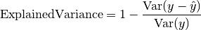
$\text{ExplainedVariance} = 1 - \frac{\text{Var}(y - \hat{y})}{\text{Var}(y)}$

Where $y$ is a tensor of target values, and $\hat{y}$ is a tensor of predictions.

Forward accepts

preds (float tensor): (N,) or (N, ...) (multioutput)
target (long tensor): (N,) or (N, ...) (multioutput)

In the case of multioutput, as default the variances will be uniformly averaged over the additional dimensions. Please see argument multioutput for changing this behavior.

Parameters

multioutput¶ (str) –
Defines aggregation in the case of multiple output scores. Can be one of the following strings (default is ‘uniform_average’.):
- ’raw_values’ returns full set of scores
- ’uniform_average’ scores are uniformly averaged
- ’variance_weighted’ scores are weighted by their individual variances
compute_on_step¶ (bool) – Forward only calls update() and return None if this is set to False. default: True
dist_sync_on_step¶ (bool) – Synchronize metric state across processes at each forward() before returning the value at the step. default: False
process_group¶ (Optional[Any]) – Specify the process group on which synchronization is called. default: None (which selects the entire world)

Example

>>> from pytorch_lightning.metrics import ExplainedVariance
>>> target = torch.tensor([3, -0.5, 2, 7])
>>> preds = torch.tensor([2.5, 0.0, 2, 8])
>>> explained_variance = ExplainedVariance()
>>> explained_variance(preds, target)
tensor(0.9572)

>>> target = torch.tensor([[0.5, 1], [-1, 1], [7, -6]])
>>> preds = torch.tensor([[0, 2], [-1, 2], [8, -5]])
>>> explained_variance = ExplainedVariance(multioutput='raw_values')
>>> explained_variance(preds, target)
tensor([0.9677, 1.0000])

compute()[source]: Computes explained variance over state.

update(preds, target)[source]

Update state with predictions and targets.

Parameters

preds¶ (Tensor) – Predictions from model
target¶ (Tensor) – Ground truth values

MeanAbsoluteError¶

class pytorch_lightning.metrics.regression.MeanAbsoluteError(compute_on_step=True, dist_sync_on_step=False, process_group=None, dist_sync_fn=None)[source]

Bases: torchmetrics.

Computes mean absolute error (MAE):

$\text{MAE} = \frac{1}{N}\sum_i^N | y_i - \hat{y_i} |$

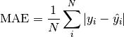
Where $y$ is a tensor of target values, and $\hat{y}$ is a tensor of predictions.

Parameters

compute_on_step¶ (bool) – Forward only calls update() and return None if this is set to False. default: True
dist_sync_on_step¶ (bool) – Synchronize metric state across processes at each forward() before returning the value at the step. default: False
process_group¶ (Optional[Any]) – Specify the process group on which synchronization is called. default: None (which selects the entire world)

Example

>>> from pytorch_lightning.metrics import MeanAbsoluteError
>>> target = torch.tensor([3.0, -0.5, 2.0, 7.0])
>>> preds = torch.tensor([2.5, 0.0, 2.0, 8.0])
>>> mean_absolute_error = MeanAbsoluteError()
>>> mean_absolute_error(preds, target)
tensor(0.5000)

compute()[source]: Computes mean absolute error over state.

update(preds, target)[source]

Update state with predictions and targets.

Parameters

preds¶ (Tensor) – Predictions from model
target¶ (Tensor) – Ground truth values

MeanSquaredError¶

class pytorch_lightning.metrics.regression.MeanSquaredError(compute_on_step=True, dist_sync_on_step=False, process_group=None, dist_sync_fn=None)[source]

Bases: torchmetrics.

Computes mean squared error (MSE):

$\text{MSE} = \frac{1}{N}\sum_i^N(y_i - \hat{y_i})^2$

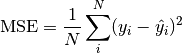
Where $y$ is a tensor of target values, and $\hat{y}$ is a tensor of predictions.

Parameters

compute_on_step¶ (bool) – Forward only calls update() and return None if this is set to False. default: True
dist_sync_on_step¶ (bool) – Synchronize metric state across processes at each forward() before returning the value at the step. default: False
process_group¶ (Optional[Any]) – Specify the process group on which synchronization is called. default: None (which selects the entire world)

Example

>>> from pytorch_lightning.metrics import MeanSquaredError
>>> target = torch.tensor([2.5, 5.0, 4.0, 8.0])
>>> preds = torch.tensor([3.0, 5.0, 2.5, 7.0])
>>> mean_squared_error = MeanSquaredError()
>>> mean_squared_error(preds, target)
tensor(0.8750)

compute()[source]: Computes mean squared error over state.

update(preds, target)[source]

Update state with predictions and targets.

Parameters

preds¶ (Tensor) – Predictions from model
target¶ (Tensor) – Ground truth values

MeanSquaredLogError¶

class pytorch_lightning.metrics.regression.MeanSquaredLogError(compute_on_step=True, dist_sync_on_step=False, process_group=None, dist_sync_fn=None)[source]

Bases: torchmetrics.

Computes mean squared logarithmic error (MSLE):

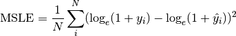
$\text{MSLE} = \frac{1}{N}\sum_i^N (\log_e(1 + y_i) - \log_e(1 + \hat{y_i}))^2$

Where $y$ is a tensor of target values, and $\hat{y}$ is a tensor of predictions.

Parameters

compute_on_step¶ (bool) – Forward only calls update() and return None if this is set to False. default: True
dist_sync_on_step¶ (bool) – Synchronize metric state across processes at each forward() before returning the value at the step. default: False
process_group¶ (Optional[Any]) – Specify the process group on which synchronization is called. default: None (which selects the entire world)

Example

>>> from pytorch_lightning.metrics import MeanSquaredLogError
>>> target = torch.tensor([2.5, 5, 4, 8])
>>> preds = torch.tensor([3, 5, 2.5, 7])
>>> mean_squared_log_error = MeanSquaredLogError()
>>> mean_squared_log_error(preds, target)
tensor(0.0397)

compute()[source]: Compute mean squared logarithmic error over state.

update(preds, target)[source]

Update state with predictions and targets.

Parameters

preds¶ (Tensor) – Predictions from model
target¶ (Tensor) – Ground truth values

PSNR¶

class pytorch_lightning.metrics.regression.PSNR(data_range=None, base=10.0, reduction='elementwise_mean', dim=None, compute_on_step=True, dist_sync_on_step=False, process_group=None)[source]

Bases: torchmetrics.

Computes peak signal-to-noise ratio (PSNR):

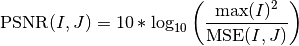
$\text{PSNR}(I, J) = 10 * \log_{10} \left(\frac{\max(I)^2}{\text{MSE}(I, J)}\right)$

Where $\text{MSE}$ denotes the mean-squared-error function.

Parameters

data_range¶ (Optional[float]) – the range of the data. If None, it is determined from the data (max - min). The data_range must be given when dim is not None.
base¶ (float) – a base of a logarithm to use (default: 10)
reduction¶ (str) –
a method to reduce metric score over labels.
- 'elementwise_mean': takes the mean (default)
- 'sum': takes the sum
- 'none': no reduction will be applied
dim¶ (Union[int, Tuple[int, …], None]) – Dimensions to reduce PSNR scores over, provided as either an integer or a list of integers. Default is None meaning scores will be reduced across all dimensions and all batches.
compute_on_step¶ (bool) – Forward only calls update() and return None if this is set to False. default: True
dist_sync_on_step¶ (bool) – Synchronize metric state across processes at each forward() before returning the value at the step. default: False
process_group¶ (Optional[Any]) – Specify the process group on which synchronization is called. default: None (which selects the entire world)

Example

>>> from pytorch_lightning.metrics import PSNR
>>> psnr = PSNR()
>>> preds = torch.tensor([[0.0, 1.0], [2.0, 3.0]])
>>> target = torch.tensor([[3.0, 2.0], [1.0, 0.0]])
>>> psnr(preds, target)
tensor(2.5527)

compute()[source]: Compute peak signal-to-noise ratio over state.

update(preds, target)[source]

Update state with predictions and targets.

Parameters

preds¶ (Tensor) – Predictions from model
target¶ (Tensor) – Ground truth values

SSIM¶

class pytorch_lightning.metrics.regression.SSIM(kernel_size=(11, 11), sigma=(1.5, 1.5), reduction='elementwise_mean', data_range=None, k1=0.01, k2=0.03, compute_on_step=True, dist_sync_on_step=False, process_group=None)[source]

Bases: torchmetrics.

Computes Structual Similarity Index Measure (SSIM).

Parameters

kernel_size¶ (Sequence[int]) – size of the gaussian kernel (default: (11, 11))
sigma¶ (Sequence[float]) – Standard deviation of the gaussian kernel (default: (1.5, 1.5))
reduction¶ (str) –
a method to reduce metric score over labels.
- 'elementwise_mean': takes the mean (default)
- 'sum': takes the sum
- 'none': no reduction will be applied
data_range¶ (Optional[float]) – Range of the image. If None, it is determined from the image (max - min)
k1¶ (float) – Parameter of SSIM. Default: 0.01
k2¶ (float) – Parameter of SSIM. Default: 0.03

Returns

Tensor with SSIM score

Example

>>> from pytorch_lightning.metrics import SSIM
>>> preds = torch.rand([16, 1, 16, 16])
>>> target = preds * 0.75
>>> ssim = SSIM()
>>> ssim(preds, target)
tensor(0.9219)

compute()[source]: Computes explained variance over state.

update(preds, target)[source]

Update state with predictions and targets.

Parameters

preds¶ (Tensor) – Predictions from model
target¶ (Tensor) – Ground truth values

R2Score¶

class pytorch_lightning.metrics.regression.R2Score(num_outputs=1, adjusted=0, multioutput='uniform_average', compute_on_step=True, dist_sync_on_step=False, process_group=None, dist_sync_fn=None)[source]

Bases: torchmetrics.

Computes r2 score also known as coefficient of determination:

$R^2 = 1 - \frac{SS_res}{SS_tot}$

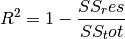
where $SS_res=\sum_i (y_i - f(x_i))^2$ is the sum of residual squares, and $SS_tot=\sum_i (y_i - \bar{y})^2$ is total sum of squares. Can also calculate adjusted r2 score given by

$R^2_adj = 1 - \frac{(1-R^2)(n-1)}{n-k-1}$

where the parameter $k$ (the number of independent regressors) should be provided as the adjusted argument.

Forward accepts

preds (float tensor): (N,) or (N, M) (multioutput)
target (float tensor): (N,) or (N, M) (multioutput)

In the case of multioutput, as default the variances will be uniformly averaged over the additional dimensions. Please see argument multioutput for changing this behavior.

Parameters

num_outputs¶ (int) – Number of outputs in multioutput setting (default is 1)
adjusted¶ (int) – number of independent regressors for calculating adjusted r2 score. Default 0 (standard r2 score).
multioutput¶ (str) –
Defines aggregation in the case of multiple output scores. Can be one of the following strings (default is 'uniform_average'.):
- 'raw_values' returns full set of scores
- 'uniform_average' scores are uniformly averaged
- 'variance_weighted' scores are weighted by their individual variances
compute_on_step¶ (bool) – Forward only calls update() and return None if this is set to False. default: True
dist_sync_on_step¶ (bool) – Synchronize metric state across processes at each forward() before returning the value at the step. default: False
process_group¶ (Optional[Any]) – Specify the process group on which synchronization is called. default: None (which selects the entire world)

Example

>>> from pytorch_lightning.metrics import R2Score
>>> target = torch.tensor([3, -0.5, 2, 7])
>>> preds = torch.tensor([2.5, 0.0, 2, 8])
>>> r2score = R2Score()
>>> r2score(preds, target)
tensor(0.9486)

>>> target = torch.tensor([[0.5, 1], [-1, 1], [7, -6]])
>>> preds = torch.tensor([[0, 2], [-1, 2], [8, -5]])
>>> r2score = R2Score(num_outputs=2, multioutput='raw_values')
>>> r2score(preds, target)
tensor([0.9654, 0.9082])

compute()[source]

Computes r2 score over the metric states.

Return type: Tensor

update(preds, target)[source]

Update state with predictions and targets.

Parameters

preds¶ (Tensor) – Predictions from model
target¶ (Tensor) – Ground truth values

Functional Metrics (Regression)¶

explained_variance [func]¶

pytorch_lightning.metrics.functional.explained_variance(preds, target, multioutput='uniform_average')[source]

Computes explained variance.

Parameters

preds¶ (Tensor) – estimated labels
target¶ (Tensor) – ground truth labels
multioutput¶ (str) –
Defines aggregation in the case of multiple output scores. Can be one of the following strings (default is ‘uniform_average’.):
- ’raw_values’ returns full set of scores
- ’uniform_average’ scores are uniformly averaged
- ’variance_weighted’ scores are weighted by their individual variances

Example

>>> from pytorch_lightning.metrics.functional import explained_variance
>>> target = torch.tensor([3, -0.5, 2, 7])
>>> preds = torch.tensor([2.5, 0.0, 2, 8])
>>> explained_variance(preds, target)
tensor(0.9572)

>>> target = torch.tensor([[0.5, 1], [-1, 1], [7, -6]])
>>> preds = torch.tensor([[0, 2], [-1, 2], [8, -5]])
>>> explained_variance(preds, target, multioutput='raw_values')
tensor([0.9677, 1.0000])

Return type: Union[Tensor, Sequence[Tensor]]

image_gradients [func]¶

pytorch_lightning.metrics.functional.image_gradients(img)[source]

Computes the gradients of a given image using finite difference

Parameters: img¶ (Tensor) – An (N, C, H, W) input tensor where C is the number of image channels
Return type: Tuple[Tensor, Tensor]
Returns: Tuple of (dy, dx) with each gradient of shape [N, C, H, W]

Example

>>> image = torch.arange(0, 1*1*5*5, dtype=torch.float32)
>>> image = torch.reshape(image, (1, 1, 5, 5))
>>> dy, dx = image_gradients(image)
>>> dy[0, 0, :, :]
tensor([[5., 5., 5., 5., 5.],
        [5., 5., 5., 5., 5.],
        [5., 5., 5., 5., 5.],
        [5., 5., 5., 5., 5.],
        [0., 0., 0., 0., 0.]])

Note

The implementation follows the 1-step finite difference method as followed by the TF implementation. The values are organized such that the gradient of [I(x+1, y)-[I(x, y)]] are at the (x, y) location

mean_absolute_error [func]¶

pytorch_lightning.metrics.functional.mean_absolute_error(preds, target)[source]

Computes mean absolute error

Parameters

pred¶ – estimated labels
target¶ (Tensor) – ground truth labels

Return type

Tensor

Returns

Tensor with MAE

Example

>>> x = torch.tensor([0., 1, 2, 3])
>>> y = torch.tensor([0., 1, 2, 2])
>>> mean_absolute_error(x, y)
tensor(0.2500)

mean_squared_error [func]¶

pytorch_lightning.metrics.functional.mean_squared_error(preds, target)[source]

Computes mean squared error

Parameters

preds¶ (Tensor) – estimated labels
target¶ (Tensor) – ground truth labels

Return type

Tensor

Returns

Tensor with MSE

Example

>>> x = torch.tensor([0., 1, 2, 3])
>>> y = torch.tensor([0., 1, 2, 2])
>>> mean_squared_error(x, y)
tensor(0.2500)

mean_squared_log_error [func]¶

pytorch_lightning.metrics.functional.mean_squared_log_error(preds, target)[source]

Computes mean squared log error

Parameters

preds¶ (Tensor) – estimated labels
target¶ (Tensor) – ground truth labels

Return type

Tensor

Returns

Tensor with RMSLE

Example

>>> x = torch.tensor([0., 1, 2, 3])
>>> y = torch.tensor([0., 1, 2, 2])
>>> mean_squared_log_error(x, y)
tensor(0.0207)

psnr [func]¶

pytorch_lightning.metrics.functional.psnr(preds, target, data_range=None, base=10.0, reduction='elementwise_mean', dim=None)[source]

Computes the peak signal-to-noise ratio

Parameters

preds¶ (Tensor) – estimated signal
target¶ (Tensor) – groun truth signal
data_range¶ (Optional[float]) – the range of the data. If None, it is determined from the data (max - min). data_range must be given when dim is not None.
base¶ (float) – a base of a logarithm to use (default: 10)
reduction¶ (str) –
a method to reduce metric score over labels.
- 'elementwise_mean': takes the mean (default)
- 'sum': takes the sum
- 'none': no reduction will be applied
dim¶ (Union[int, Tuple[int, …], None]) – Dimensions to reduce PSNR scores over provided as either an integer or a list of integers. Default is None meaning scores will be reduced across all dimensions.

Return type

Tensor

Returns

Tensor with PSNR score

Example

>>> pred = torch.tensor([[0.0, 1.0], [2.0, 3.0]])
>>> target = torch.tensor([[3.0, 2.0], [1.0, 0.0]])
>>> psnr(pred, target)
tensor(2.5527)

ssim [func]¶

pytorch_lightning.metrics.functional.ssim(preds, target, kernel_size=(11, 11), sigma=(1.5, 1.5), reduction='elementwise_mean', data_range=None, k1=0.01, k2=0.03)[source]

Computes Structual Similarity Index Measure

Parameters

preds¶ (Tensor) – estimated image
target¶ (Tensor) – ground truth image
kernel_size¶ (Sequence[int]) – size of the gaussian kernel (default: (11, 11))
sigma¶ (Sequence[float]) – Standard deviation of the gaussian kernel (default: (1.5, 1.5))
reduction¶ (str) –
a method to reduce metric score over labels.
- 'elementwise_mean': takes the mean (default)
- 'sum': takes the sum
- 'none': no reduction will be applied
data_range¶ (Optional[float]) – Range of the image. If None, it is determined from the image (max - min)
k1¶ (float) – Parameter of SSIM. Default: 0.01
k2¶ (float) – Parameter of SSIM. Default: 0.03

Return type

Tensor

Returns

Tensor with SSIM score

Example

>>> preds = torch.rand([16, 1, 16, 16])
>>> target = preds * 0.75
>>> ssim(preds, target)
tensor(0.9219)

r2score [func]¶

pytorch_lightning.metrics.functional.r2score(preds, target, adjusted=0, multioutput='uniform_average')[source]

Computes r2 score also known as coefficient of determination:

$R^2 = 1 - \frac{SS_res}{SS_tot}$

where $SS_res=\sum_i (y_i - f(x_i))^2$ is the sum of residual squares, and $SS_tot=\sum_i (y_i - \bar{y})^2$ is total sum of squares. Can also calculate adjusted r2 score given by

$R^2_adj = 1 - \frac{(1-R^2)(n-1)}{n-k-1}$

where the parameter $k$ (the number of independent regressors) should be provided as the adjusted argument.

Parameters

preds¶ (Tensor) – estimated labels
target¶ (Tensor) – ground truth labels
adjusted¶ (int) – number of independent regressors for calculating adjusted r2 score. Default 0 (standard r2 score).
multioutput¶ (str) –
Defines aggregation in the case of multiple output scores. Can be one of the following strings (default is 'uniform_average'.):
- 'raw_values' returns full set of scores
- 'uniform_average' scores are uniformly averaged
- 'variance_weighted' scores are weighted by their individual variances

Example

>>> from pytorch_lightning.metrics.functional import r2score
>>> target = torch.tensor([3, -0.5, 2, 7])
>>> preds = torch.tensor([2.5, 0.0, 2, 8])
>>> r2score(preds, target)
tensor(0.9486)

>>> target = torch.tensor([[0.5, 1], [-1, 1], [7, -6]])
>>> preds = torch.tensor([[0, 2], [-1, 2], [8, -5]])
>>> r2score(preds, target, multioutput='raw_values')
tensor([0.9654, 0.9082])

Return type: Tensor

NLP¶

bleu_score [func]¶

pytorch_lightning.metrics.functional.nlp.bleu_score(translate_corpus, reference_corpus, n_gram=4, smooth=False)[source]

Calculate BLEU score of machine translated text with one or more references

Parameters

translate_corpus¶ (Sequence[str]) – An iterable of machine translated corpus
reference_corpus¶ (Sequence[str]) – An iterable of iterables of reference corpus
n_gram¶ (int) – Gram value ranged from 1 to 4 (Default 4)
smooth¶ (bool) – Whether or not to apply smoothing – Lin et al. 2004

Return type

Tensor

Returns

Tensor with BLEU Score

Example

>>> translate_corpus = ['the cat is on the mat'.split()]
>>> reference_corpus = [['there is a cat on the mat'.split(), 'a cat is on the mat'.split()]]
>>> bleu_score(translate_corpus, reference_corpus)
tensor(0.7598)

Pairwise¶

embedding_similarity [func]¶

pytorch_lightning.metrics.functional.self_supervised.embedding_similarity(batch, similarity='cosine', reduction='none', zero_diagonal=True)[source]

Computes representation similarity

Example

>>> embeddings = torch.tensor([[1., 2., 3., 4.], [1., 2., 3., 4.], [4., 5., 6., 7.]])
>>> embedding_similarity(embeddings)
tensor([[0.0000, 1.0000, 0.9759],
        [1.0000, 0.0000, 0.9759],
        [0.9759, 0.9759, 0.0000]])

Parameters

batch¶ (Tensor) – (batch, dim)
similarity¶ (str) – ‘dot’ or ‘cosine’
reduction¶ (str) – ‘none’, ‘sum’, ‘mean’ (all along dim -1)
zero_diagonal¶ (bool) – if True, the diagonals are set to zero

Return type

Tensor

Returns

A square matrix (batch, batch) with the similarity scores between all elements If sum or mean are used, then returns (b, 1) with the reduced value for each row